Validation and Performance

This page separates two questions that are easy to mix together:

• Validation: does a field–window estimator recover the expected statistic, and does it converge when the numerical controls are tightened?

• Performance: once the estimator is fixed, which part of the workflow sets the runtime and memory footprint?

The validation figures, timing table, and CPU/GPU memory comparison are all generated from the current grouped jobs under tests/. They therefore form one internally consistent benchmark set rather than mixing results from different runs.

Reference Data

Unless stated otherwise, the validation examples use the Quijote fiducial-cosmology halo catalogue from realisation 8000, snapshot 004 (z = 0):

• 406,728 FoF haloes in a periodic cube of side 1000 h^-1 Mpc;

• the db2 scaling-function basis;

• J = 8 for the main tests, with selected J = 9 comparisons;

• the plane-parallel approximation for redshift-space measurements.

These are controlled algorithm tests, not a complete survey-analysis recipe. Survey masks and spatially varying selection functions require an explicit random catalogue or random SFCField.

Numerical Validation

Anisotropic 2PCF

The same Corr2PCF task can measure real- and redshift-space fields by changing the input SFCField while keeping the binning-window family fixed. The plot below maps \(s^2\xi(s,\mu)\) to the \((s_\perp,s_\parallel)\) plane. Joining two measurements at \(s_\perp=0\) makes the line-of-sight response immediately visible and also provides a compact check of tracer weighting.

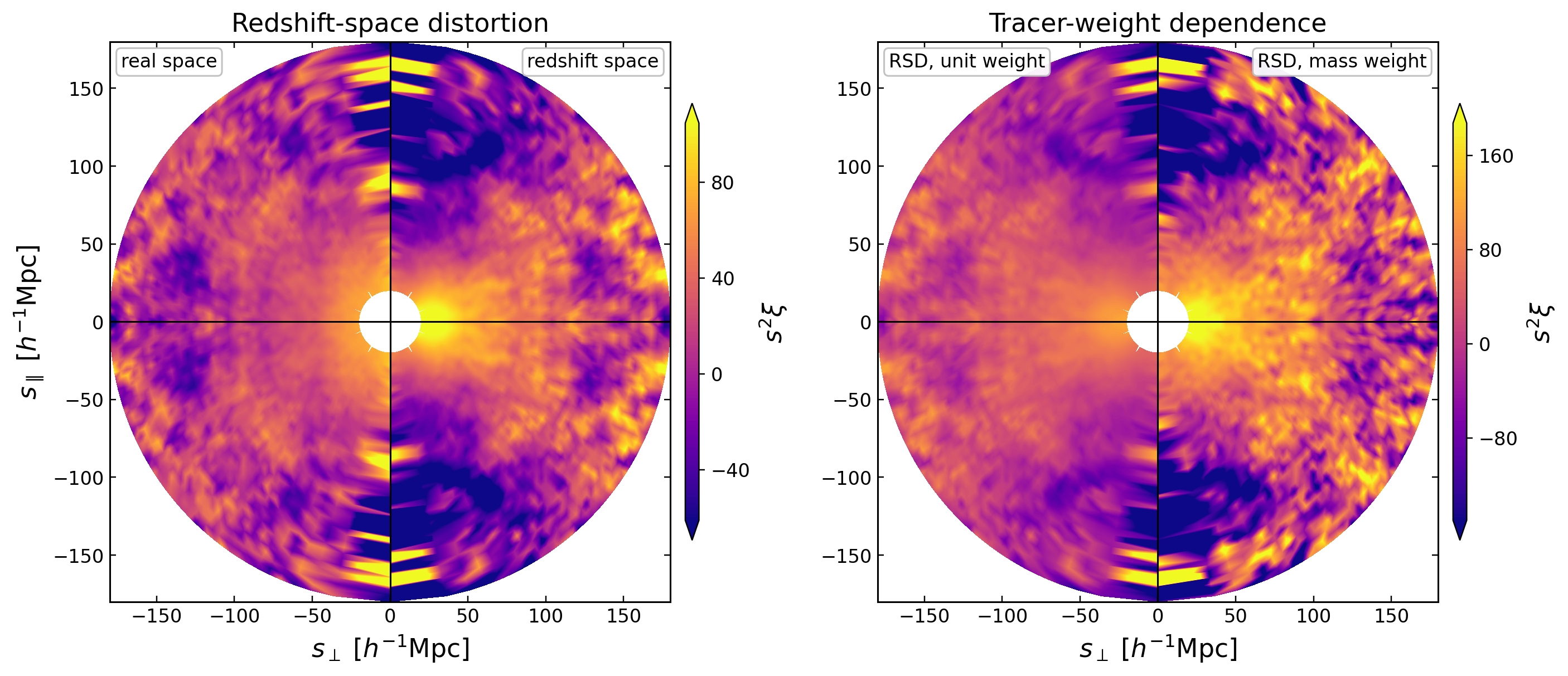
Current grouped-test outputs. Left: real space and unit-weight redshift space. Right: unit- and mass-weighted redshift space. The two halves of each circle share a colour normalization, while the two panels have separate colour bars because mass weighting has a larger dynamic range. The white centre excludes \(s<20\,h^{-1}{\rm Mpc}\).

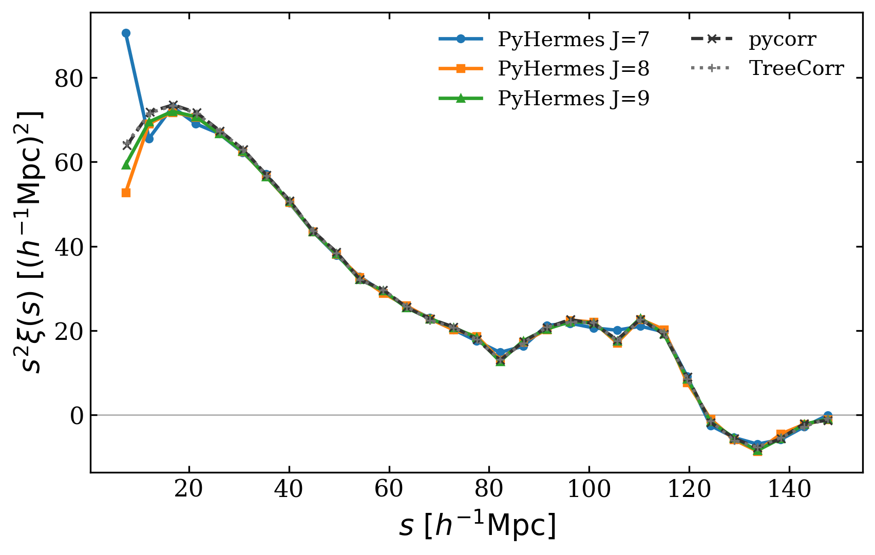
For an independent estimator-level check, the paper compares the isotropic Hermes result with direct periodic pair counting. Agreement improves with increasing J and is best interpreted only above the effective resolution scale of the reconstructed field.

Standard 3PCF

The conventional Corr3PCF task estimates translational and rotational averages by Monte Carlo sampling. Convergence must therefore be checked in n_rot rather than inferred from one visually smooth curve. In the current test, the low-rotation result fluctuates visibly while the curves and their RMS difference settle rapidly as n_rot increases.

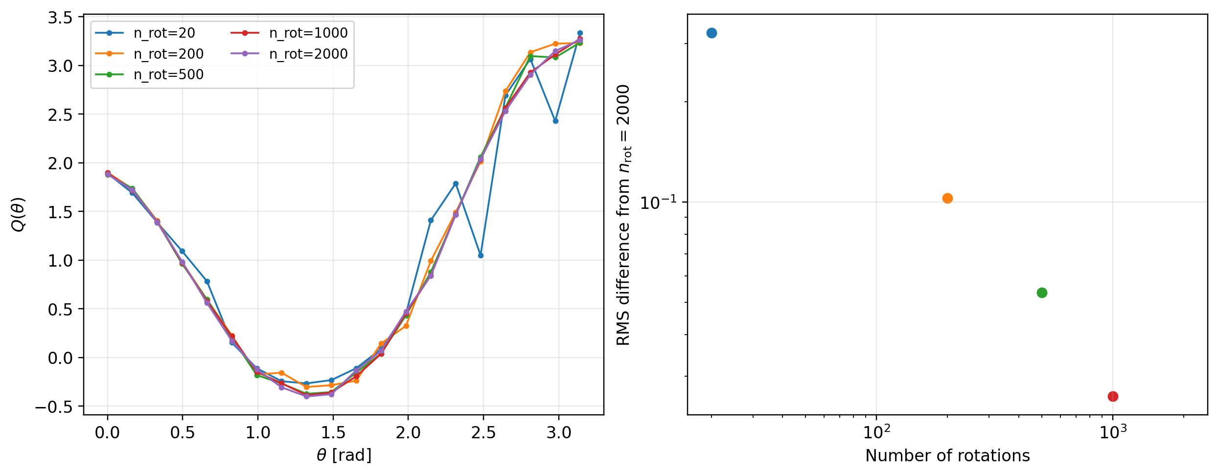
Left: \(Q(\theta)\) for several rotation counts. Right: RMS difference from the n_rot = 2000 result.

3PCF Multipoles

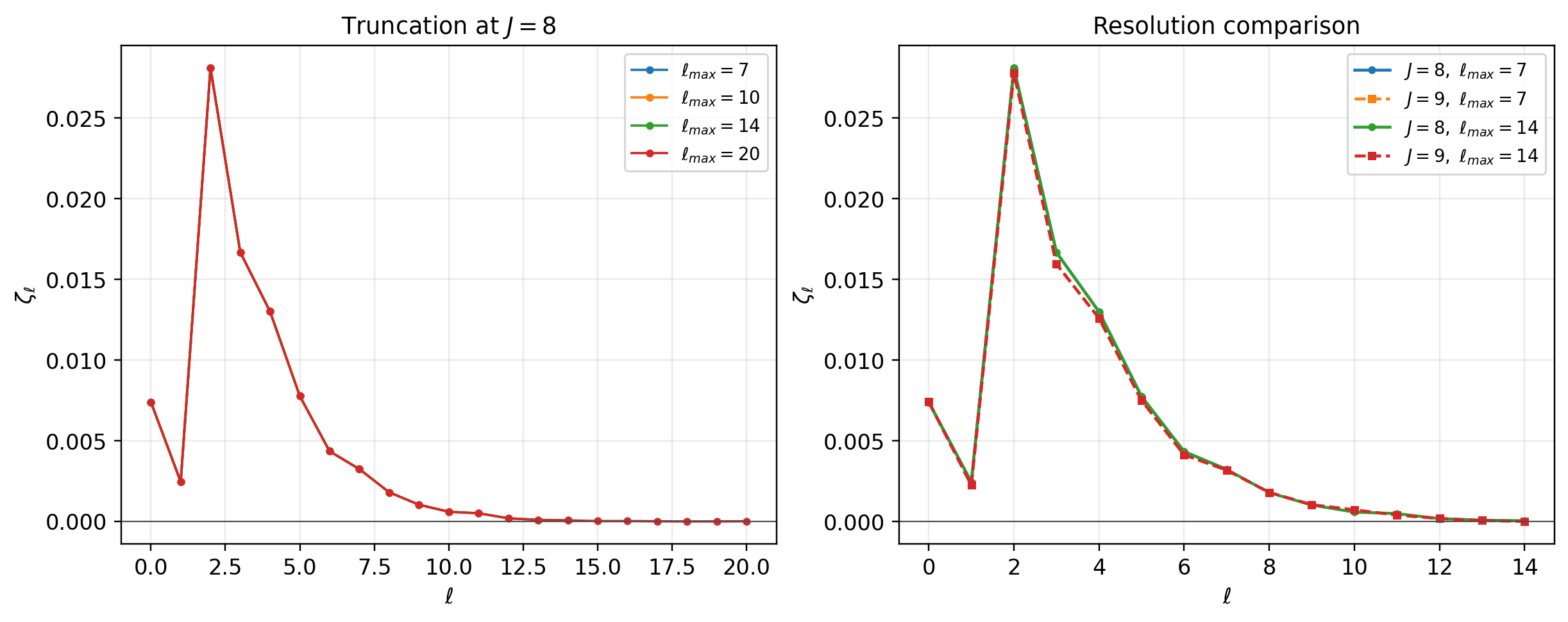
Multipole measurements have two separate convergence controls. lmax truncates the angular expansion, while J controls the MRA field resolution. The left panel below verifies that increasing lmax appends higher orders without changing the already computed low-order multipoles. The right panel compares those common modes between J = 8 and J = 9.

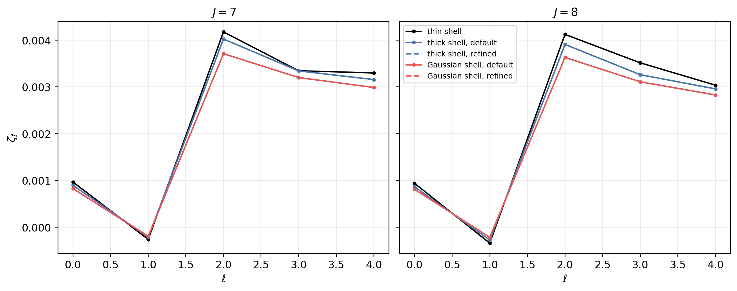
For non-shell radial profiles, PyHermes tabulates the required radial transform. The default and refined tables should agree before a profile is used for production measurements. The following check covers the thin-shell analytic path and the numerical thick- and Gaussian-shell paths.

An Ensemble-Level Check

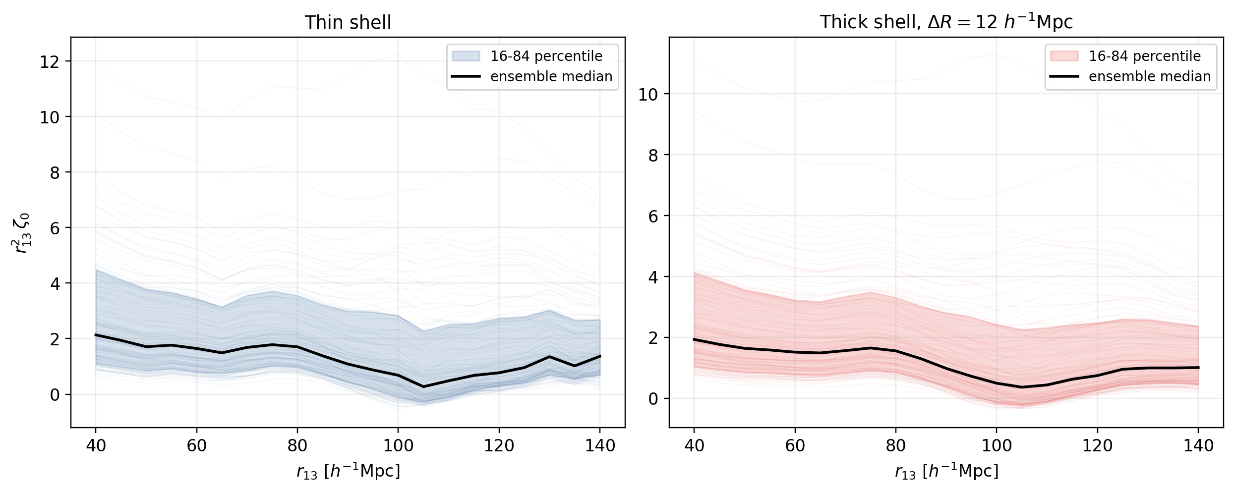
The Kun scan provides a larger application test: r12 = 20 h^-1 Mpc is held fixed while r13 varies. The 129 mocks used here span different cosmological parameters. Their spread is therefore not a covariance estimate for one cosmology; it is shown to inspect the stability of the full projection and monopole pipeline over a deliberately broad simulation ensemble.

The binning profile is part of the observable, not merely a plotting choice. For one mock, widening a finite shell or increasing the Gaussian-shell width averages a broader neighbourhood of triangle configurations:

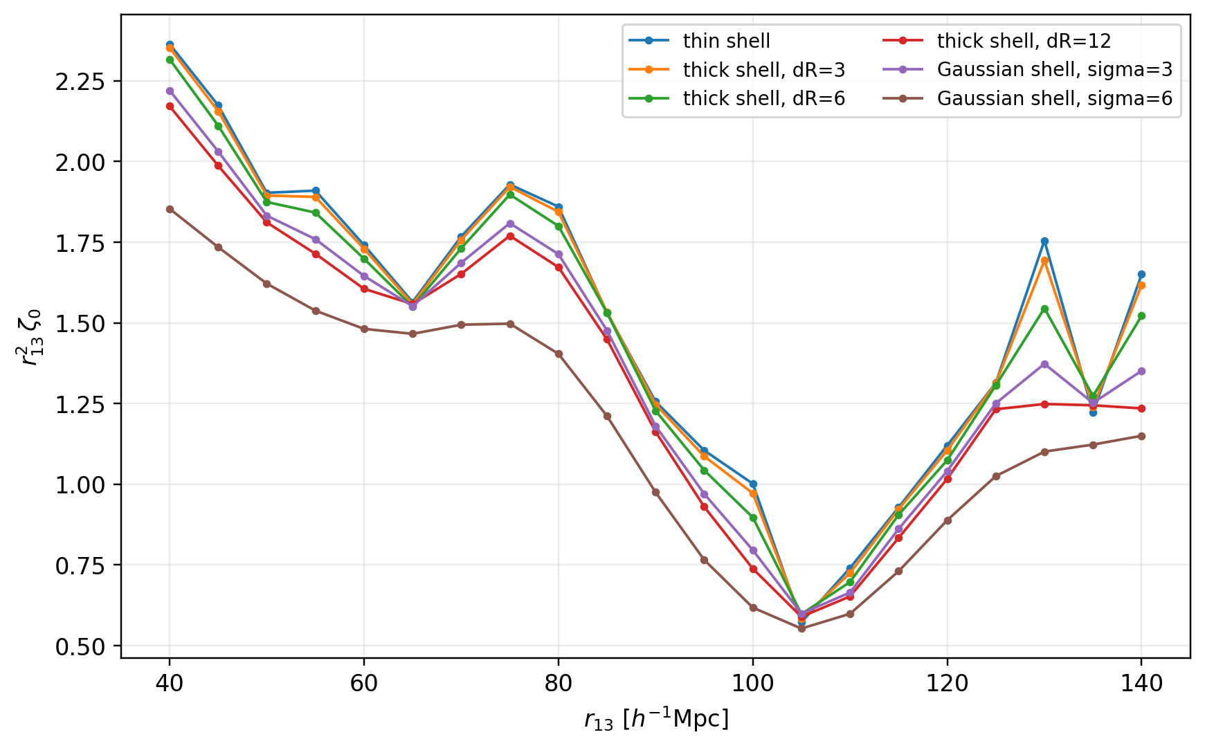
One input field and one radial scan measured with six binning profiles. The smooth variation between profiles is the expected finite-bin response.

Performance Model

The catalogue is projected once onto \(N_{\mathrm{MRA}}=2^{3J}\) coefficients. Subsequent measurements operate on fields and windows, so their leading cost depends on field resolution and the number of requested window evaluations, rather than directly on the original catalogue size.

For N_w window applications on a matching FFT grid,

\[T_{\mathrm{conv}} = \mathcal{O}\!\left(N_w N_{\mathrm{MRA}} \log N_{\mathrm{MRA}}\right).\]

The task-specific multiplicities are:

• Corr2PCF: N_s * N_mu or N_rp * N_pi sampled binning windows;

• Corr3PCF: translation samples times random rotations;

• Corr3PCFMultipole: \(N_m=(\ell_{\max}+1)(\ell_{\max}+2)/2\) explicitly evaluated non-negative-\(m\) fields.

Increasing J by one multiplies the number of three-dimensional field coefficients by eight. Since some work buffers are rank-local, a high-J job often benefits from fewer MPI ranks and more threads per rank.

Current Grouped Benchmark

The representative end-to-end jobs below use the same Quijote field and geometric setup as the validation examples. Average time is normalized by the natural sampling unit of each estimator: one \((s,\mu)\) binning window for the 2PCF and one centre–rotation–angle combination for the standard 3PCF. Memory is the Slurm batch-step MaxRSS and therefore excludes GPU device memory.

Representative 2PCF and standard-3PCF jobs

Product	Representative setup	J	Parallel	Task total	Average time	MaxRSS
\(DD(s,\mu)\)	Ring binning windows, 46 x 51 samples	8	8 x 8	119.7 s	51.0 ms/sample	8.7 GiB
\(DDD(\theta;r_{12},r_{13})\)	Particle centres, Ncen=406728, n_rot=1000, n_theta=20	8	16 x 8	84.0 s	10.3 ns/comb.	11.3 GiB
\(DDD(\theta;r_{12},r_{13})\)	Box-random centres, Ncen=8e6, n_rot=200, n_theta=20	8	16 x 8	280.6 s	8.77 ns/comb.	21.2 GiB

The CPU measurements used two AMD EPYC 9754 processors (256 physical cores in total). GPU measurements used one NVIDIA GeForce RTX 4090 with CUDA 12.4. ranks x threads below describes the CPU layout; GPU jobs use the same CPU-side convolution layout and an (8, 8, 8) CUDA block for the final contraction.

The multipole table reports the same five configurations on both backends. Convolution + MPI is the multipole-loop residual after subtracting the final contraction; the two contributions are kept together because their critical paths overlap. Task total additionally includes input, setup, and output overhead.

Current 3PCF-multipole CPU/GPU benchmark

J	lmax	\(N_m\)	Backend	Parallel	Convolution + MPI [s]	Sum [s]	Task total [s]	MaxRSS [GiB]
8	7	36	CPU	24 x 4	23.5	34.4	62.8	19.2
8	7	36	GPU	24 x 4	21.9	8.3	35.3	17.4
8	14	120	CPU	24 x 4	86.0	113.0	204.0	19.1
8	14	120	GPU	24 x 4	80.3	26.7	112.2	18.0
8	20	231	CPU	24 x 4	180.6	238.7	424.3	19.4
8	20	231	GPU	24 x 4	178.5	51.1	234.6	17.8
9	7	36	CPU	12 x 8	152.0	274.7	445.2	66.9
9	7	36	GPU	12 x 8	156.5	62.1	234.3	61.5
9	14	120	CPU	12 x 8	613.0	903.6	1528.4	65.9
9	14	120	GPU	12 x 8	616.2	206.0	833.9	61.5

CPU and GPU Multipole Backends

The backend switch applies to the final multipole-field contraction. FFT window convolutions and MPI communication remain CPU-side for both backends. Consequently, the GPU strongly accelerates the contraction stage, while the end-to-end gain is bounded by the unchanged field and communication stages.

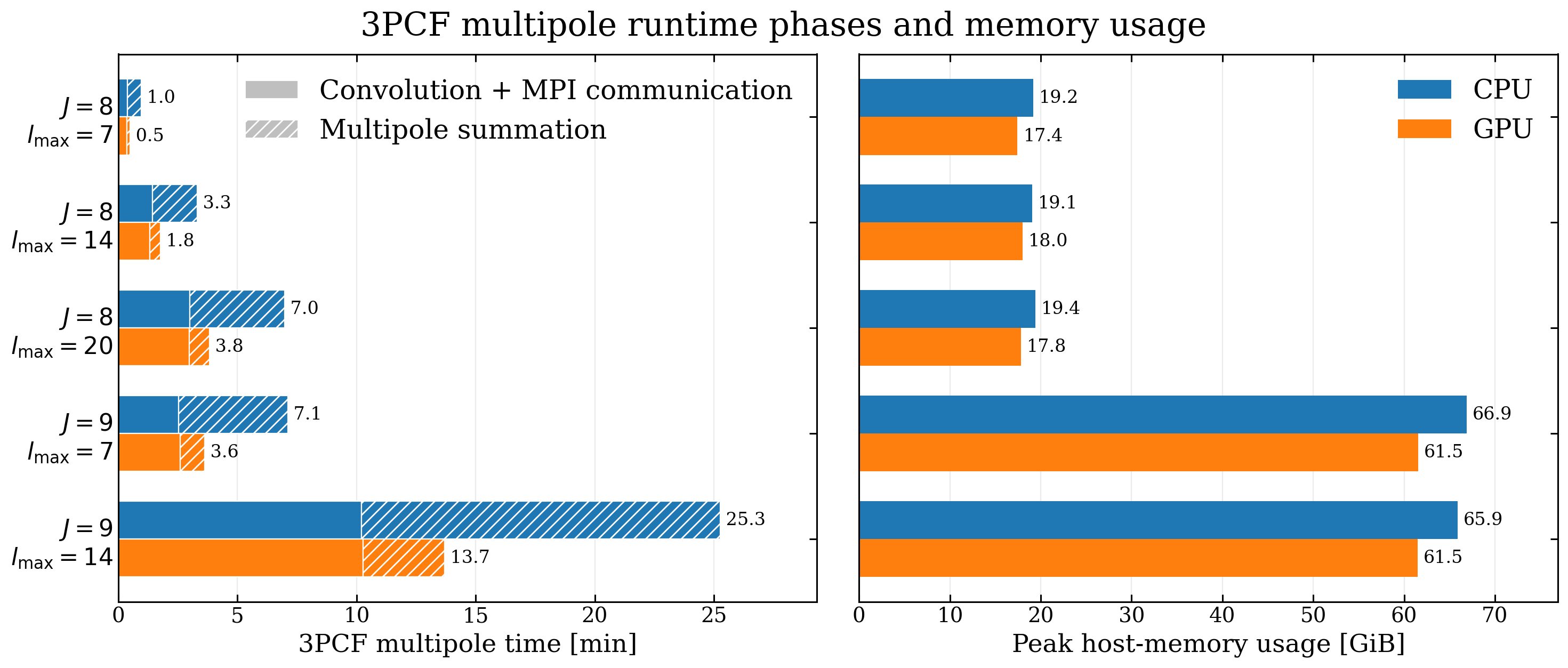
Current grouped benchmark using 24 x 4 at J=8 and 12 x 8 at J=9. Left: multipole-loop wall time split into field/MPI work and the backend-selected contraction. Right: Slurm MaxRSS host memory; GPU device memory is not included.

The CPU and GPU products agree to relative \(L_2\) differences of 9.5e-15--2.2e-14. Across the five configurations, GPU contraction is 4.1--4.7x faster and complete task time is 1.8--1.9x faster. The smaller end-to-end ratio is expected because only the contraction is offloaded. At fixed J, host memory depends only weakly on lmax because multipole windows are generated and processed sequentially. The GPU jobs use 5.6--9.1% less host memory in these measurements, but this comparison does not include device memory and is not a total CPU-plus-GPU footprint. Increasing J has the much larger memory effect: it multiplies the three-dimensional coefficient count by eight. Using fewer MPI ranks at J=9 limits the observed host-memory increase to approximately 3.4--3.5x.

Reproducing the Checks

The public examples/notebooks directory contains the user-facing workflows. For maintainers, the current grouped outputs are analysed by five deliberately small notebooks:

• tests/notebooks/docs_2pcf_results.ipynb;

• tests/notebooks/docs_3pcf_results.ipynb;

• tests/notebooks/docs_3pcf_multipole_results.ipynb;

• tests/notebooks/docs_kun_monopole_results.ipynb;

• tests/notebooks/paper_figures_performance.ipynb for the current timing and Slurm-memory table used above.

Once the grouped jobs have produced their outputs, these notebooks read the saved products rather than rerunning expensive estimators. The corresponding scripts and grouped Slurm recipes live under tests/scripts and tests/slurm. Raw logs and estimator products are treated as transient test artifacts and are intentionally not distributed with the repository. Treat absolute times as hardware-specific; convergence patterns, stage-level scaling, and same-node CPU/GPU ratios are the more portable diagnostics.