Quick start#

This is the canonical first PyHermes calculation. Starting with no local catalogue, it downloads one original Quijote FoF group_tab file, constructs a reusable SFCField, measures an isotropic 2PCF, saves both products, and plots the result. The matching notebook is available directly in the documentation; it reads the same YAML files and writes the same outputs shown here.

Run from `examples/`#

The paths in the public configurations are relative to that directory:

When working from a repository clone, install that checkout once so the commands and notebook import the code beside them rather than another PyHermes installation:

python -m pip install -e ".[plot]"

cd examples

Project the catalogue#

configs/param_sfc_projection.yaml contains the remote input and its local cache policy:

SFCProjection:
   fin:
      path: https://pyhermes.astroslacker.com/downloads/group_tab_004.0
      format: fof
      download:
         cache_path: ./data/quijote_halos/8000/groups_004/group_tab_004.0
         sha256: 4a1c6ca4f6747a70e9e552685226ecf5d678c6c97551e2caa7cc3883502eac85
      catalog_weight_key: null
      field_value_key: null
   box_size: 1000.0
   J: 8
   wavelet_mode: db2
   wavelet_level: 10
   phi_resolution: 1024
   weight_normalization: catalog
   threads: 2
   save_particle_data: true
   particle_data_path: ./output/quijote8000_snap004_particles.npz
   fout_path: ./output/quijote8000_snap004_sfc.pkl

Run the standard driver:

python scripts/run_sfc_projection.py configs/param_sfc_projection.yaml

On the first run PyHermes downloads about 33 MB, verifies its SHA256 digest, and caches it at data/quijote_halos/8000/groups_004/group_tab_004.0. Later runs use that file directly. The file header reports Nfiles = 1, so no additional FoF pieces are required. SFCProjection writes the reusable field and a compact particle companion for particle-centred tasks.

Measure the 2PCF#

The second configuration consumes exactly that field:

Corr_2PCF:
   sfc_field: ./output/quijote8000_snap004_sfc.pkl
   random: uniform
   binning_window: shell
   sampling:
      s: {min: 0.0, max: 150.0, n: 31}
   products: [dd, dr, rd, xi]
   threads: 2
   fout_path: ./output/quijote8000_snap004_2pcf.pkl

python scripts/run_2pcf.py configs/param_2pcf.yaml

random: uniform is an analytic constant reference field, so this basic run has no stochastic random catalogue or hidden random seed. The vertices receive no additional smoothing; shell supplies only the sampled radial binning operator.

Load and plot#

Task outputs are read through their public data classes:

import matplotlib.pyplot as plt
from pyhermes.io import Corr2PCFData

corr = Corr2PCFData(
    data_path="./output/quijote8000_snap004_2pcf.pkl"
)

fig, ax = plt.subplots(figsize=(7.0, 4.6))
ax.plot(corr.s, corr.s**2 * corr.xi, color="#1f77b4", lw=2.0)
ax.axhline(0.0, color="0.35", lw=0.8)
ax.set(
    xlabel=r"$s\ [h^{-1}\mathrm{Mpc}]$",
    ylabel=r"$s^2\xi(s)$",
)
ax.grid(alpha=0.25)
fig.tight_layout()
plt.show()

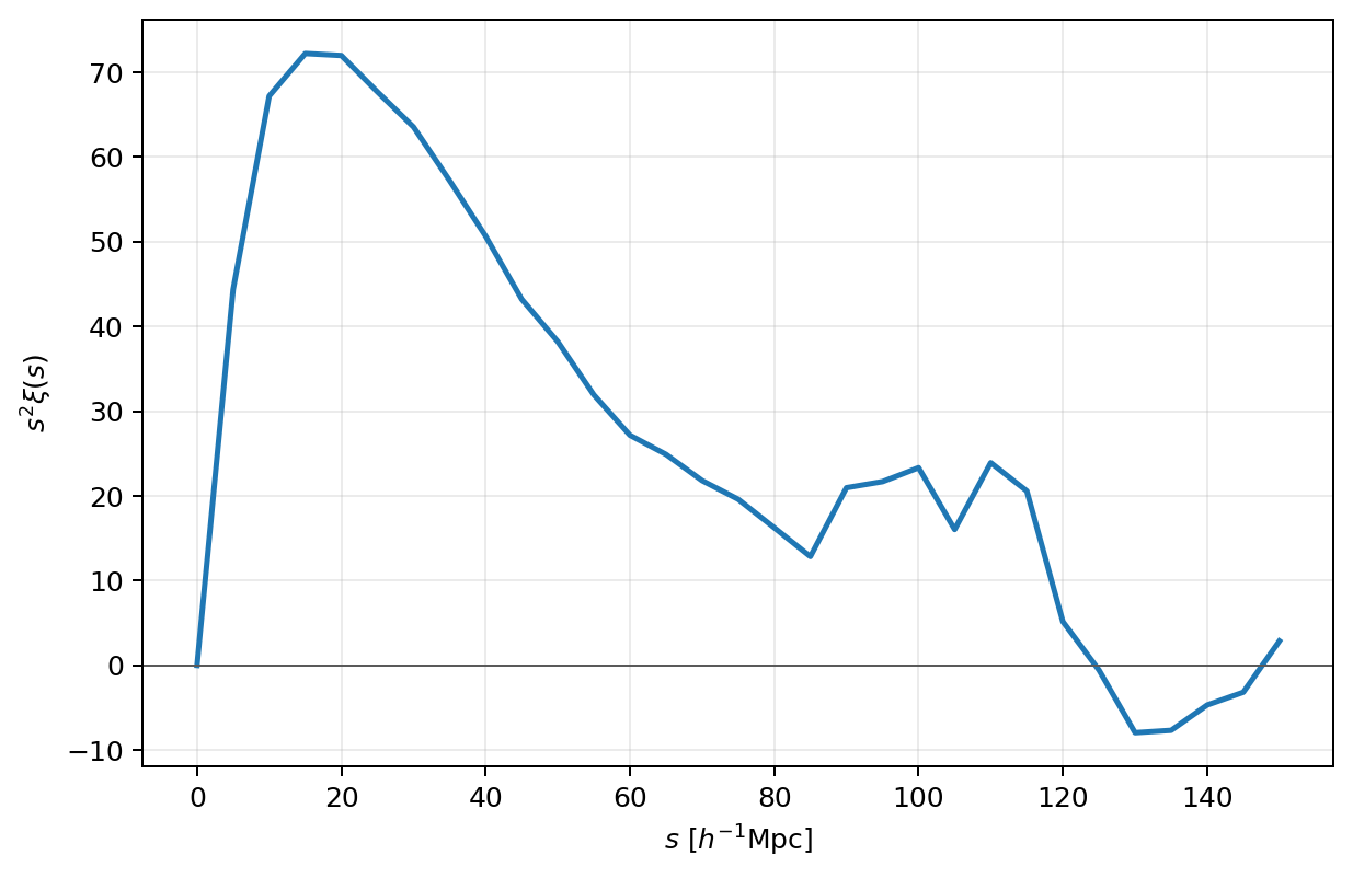
../_images/quick_start_2pcf.png — The isotropic 2PCF produced by the Quick Start YAML and notebook.#

The notebook executes these same three stages through the Python task API. There is deliberately no second set of separations, smoothing parameters, or output names to reconcile.

Where next?#

The Quick Start is the shortest complete workflow. The next three notebooks explain its reusable layers:

Particle input and conversion is the optional input-data branch. It starts from the same FoF catalogue and shows how equivalent NPZ and raw BIN catalogues can be constructed and read.
Build an SFCField develops the catalogue-to-SFCField step: weights, normalisation, resolution, redshift space, and reusable products.
Field and window operations develops the SFCField @ WindowFunc language: smoothing, custom kernels, and field algebra.

After that common foundation, choose the scientific branch that matches the question:

Physical fields from field–window operations applies differential and inverse-Laplacian windows to velocity, momentum, potential, and acceleration fields.
Counting and one-point PDFs samples fields for one-point distributions.
Two-point correlation functions extends the first 2PCF to smoothing, alternative bins, cross-correlations, and redshift-space anisotropy.
Standard 3PCF and 3PCF multipoles continue the statistics path to angular and multipole three-point measurements.

For a first top-to-bottom reading, the recommended linear order is quick_start -> particle_io -> sfc_projection -> window -> physical_fields -> counting -> corr2pcf -> corr3pcf. particle_io may be skipped when the public example catalogue is enough; the application notebooks after window are independent branches rather than strict prerequisites for one another.

The projection tutorial generates its own J=9, mass-weighted, redshift-space, and sampled-random fields. A dense dark-matter snapshot is the only advanced external product used by physical_fields.ipynb; that notebook identifies the script and Slurm job that build it.