Build an SFCField

SFCProjection is the reusable first stage of every PyHermes workflow. It projects particle positions and optional per-particle amplitudes onto the scaling-function basis and returns an SFCField.

The complete SFC projection notebook extends the Quick Start with number and mass fields, resolution comparisons, redshift-space coordinates, random fields, and reusable outputs.

Minimal YAML

The public example uses a single-file Quijote halo catalogue. A fresh run downloads and caches it automatically:

SFCProjection:
   fin:
      path: https://pyhermes.astroslacker.com/downloads/group_tab_004.0
      format: fof
      download:
         cache_path: ./data/quijote_halos/8000/groups_004/group_tab_004.0
         sha256: 4a1c6ca4f6747a70e9e552685226ecf5d678c6c97551e2caa7cc3883502eac85
      catalog_weight_key: null
      field_value_key: null
   box_size: 1000
   J: 8
   wavelet_mode: db2
   wavelet_level: 10
   phi_resolution: 1024
   weight_normalization: catalog
   threads: 2
   save_particle_data: true
   particle_data_path: ./output/quijote8000_snap004_particles.npz
   fout_path: ./output/quijote8000_snap004_sfc.pkl

Run it from examples/:

python scripts/run_sfc_projection.py configs/param_sfc_projection.yaml

or from Python:

from pyhermes.base.sfc_projection import SFCProjection
from pyhermes.param.parambase import read_param

params = read_param(config_path="./configs/param_sfc_projection.yaml")
field = SFCProjection(params).run()

In-memory catalogues

File readers are optional. The same task accepts arrays directly:

task = SFCProjection()
task.particle_pos = positions       # shape (N, 3)
task.catalog_weight = completeness # shape (N,), optional
task.field_value = mass            # shape (N,), optional
task.box_size = 1000.0
task.J = 8
task.weight_normalization = "catalog"
task.threads = 8
task.fout_path = "./output/mass_sfc.pkl"
mass_field = task.run()

Scalar weights and values are broadcast to all particles. Arrays must be finite and have one entry per position.

Catalogue weights and field values

The projected amplitude is the product catalog_weight * field_value. The two inputs have different meanings:

catalog_weight

Selection, completeness, optimal, or other catalogue weight.

field_value

The physical or statistical value carried by a particle, such as mass, a velocity component, or a mark.

For file readers, fin.catalog_weight_key and fin.field_value_key select named or indexed arrays exposed by the reader. With no keys, both factors are one.

Normalisation

weight_normalization controls the projection denominator:

Mode	Denominator	Typical use
raw	1	Raw counts or extensive physical fields
catalog	sum(catalog_weight)	Number fields and weighted means; task default
field	sum(catalog_weight * field_value)	Unit-integral marked or physical field

The output metadata records the raw sums, the selected normalisation, and the resulting field_integral. A catalogue field may later be converted without reprojecting particles:

raw_field = field.switch_weight_normalization("raw")
unit_field = field.to_unit_weight()

Choose J from the resolved scale

For a box of side box_size, the nominal MRA spacing is box_size / 2**J. In a \(1000\,h^{-1}\mathrm{Mpc}\) box:

J	Nominal spacing	Practical interpretation
7	7.8125 Mpc/h	Large-scale or inexpensive diagnostic field
8	3.90625 Mpc/h	Default scale for the paper’s main examples
9	1.953125 Mpc/h	Finer small-scale recovery at substantially higher memory cost

Use at least two resolutions for a statistic near the grid scale. More coefficients are useful only if the catalogue sampling can support them.

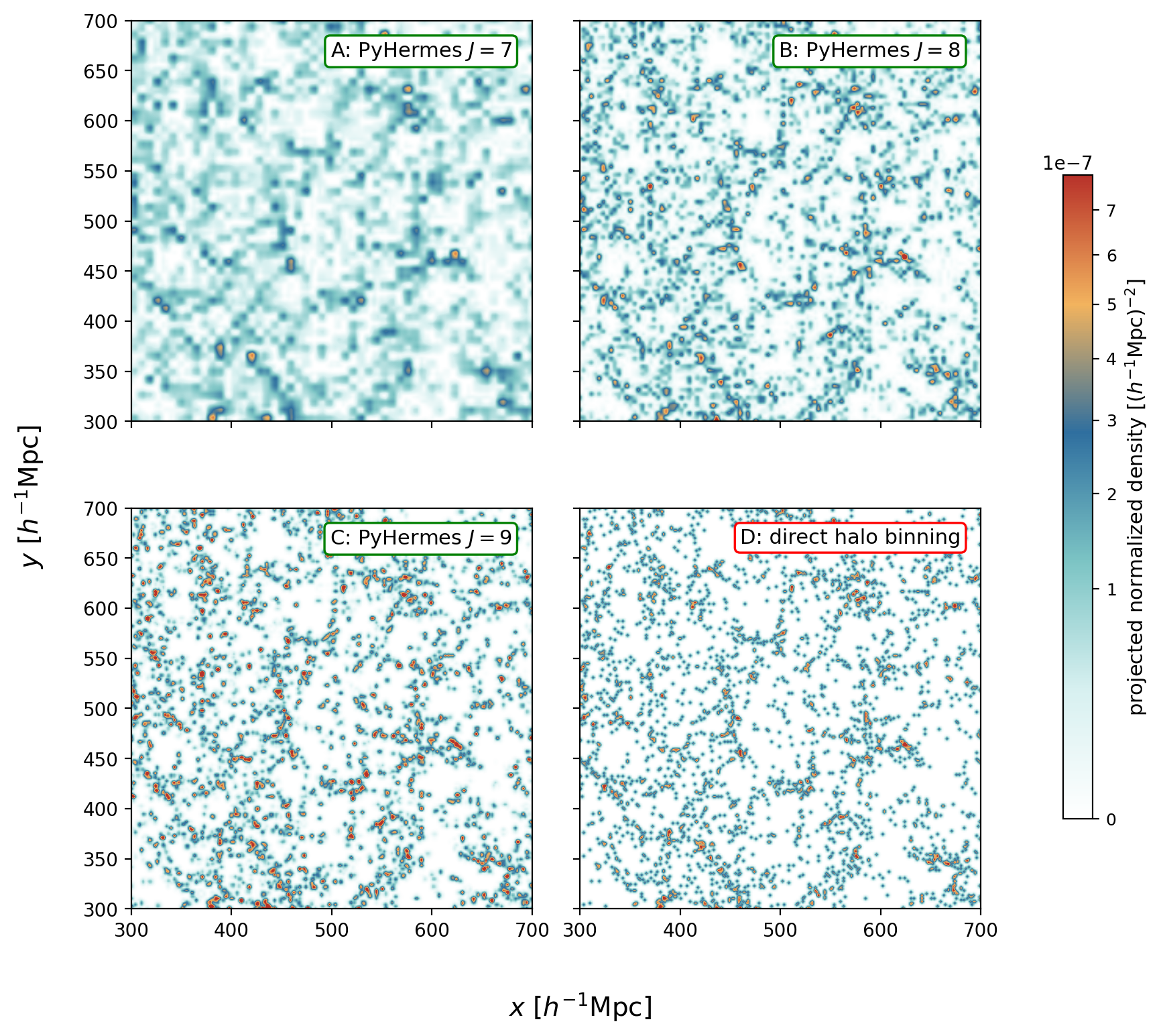
The reconstructed density converges toward finer structure as J increases. The comparison is a resolution diagnostic, not a colour-map contest.

Load and inspect a field

from pyhermes.io import SFCField

D = SFCField(
    data_path="./output/quijote8000_snap004_sfc.pkl",
    threads=8,
)
print(D.epsilon.shape)
print(D.J, D.box_size, D.wavelet_mode)
print(D.field_integral, D.weight_normalization)

Evaluate the reconstructed continuous field at arbitrary positions:

density = D.field_density_at_pos(
    sample_positions,
    value_unit="physical",
)

value_unit="physical" reports density per physical box volume; "grid" reports density per MRA-grid volume. "auto" selects physical units for catalogue fields and grid units for derived fields.

Particle data for particle-centred tasks

Corr_3PCF(center="particle") needs the primary particle positions and weights. save_particle_data: true writes a companion NPZ containing pos, catalog_weight, and field_value. The SFC metadata stores its path so get_particle_data() can recover the catalogue later.

If the original reader path remains accessible, PyHermes can reread it instead. Saving the compact companion file is usually more portable for server runs.

MPI behaviour

In a distributed projection, rank 0 reads the catalogue, partitions particles into x slabs, sends each slab to one rank, and gathers the projected slabs. The current projection implementation requires the MPI rank count to be a power of two. threads applies within every rank.

Public tutorial

The rendered notebook begins after the Quick Start and keeps the projection layer in view: configuration-driven and in-memory input, number and mass fields, reconstructed J=7/J=8/J=9 fields compared with direct halo binning, redshift-space coordinates, a matching random field, and compact companion particle datasets. It runs entirely from the public catalogue used by the Quick Start and writes the reusable products needed by the later example notebooks.

Catalogue formats and conversion are covered separately in the Particle I/O notebook and Particle input and conversion. The examples/scripts/prepare_sfc_fields.py helper produces the same field set for non-interactive or batch workflows, so it does not need to be run after the notebook.