Hermes concepts and equations#

This page is the compact mathematical map behind the task guides. It follows the notation of the Hermes paper while naming the corresponding PyHermes objects explicitly.

From a catalogue to a continuous field#

For particle positions \(\mathbf{x}_i\), catalogue weights \(w_i\), and optional particle-carried values \(q_i\), define

\[F(\mathbf{x}) = \sum_i w_i q_i\, \delta_{\mathrm D}^{3}(\mathbf{x}-\mathbf{x}_i).\]

catalog_weight supplies \(w_i\); field_value supplies \(q_i\). Unit values produce an ordinary number-density field. Mass, velocity components, marks, or other scalar values produce weighted fields without changing the projection algorithm.

At multiresolution level \(J\), PyHermes projects the catalogue onto a tensor-product scaling-function basis,

\[F_J(\mathbf{x}) = \sum_{\mathbf{l}} \epsilon_{J\mathbf{l}}\,\phi_{J\mathbf{l}}(\mathbf{x}), \qquad \epsilon_{J\mathbf{l}} = \int F(\mathbf{x}) \phi_{J\mathbf{l}}(\mathbf{x})\,d^3x.\]

The array of \(\epsilon_{J\mathbf{l}}\) is SFCField.epsilon. SFCProjection computes it directly from particle positions using the compact support of the scaling function.

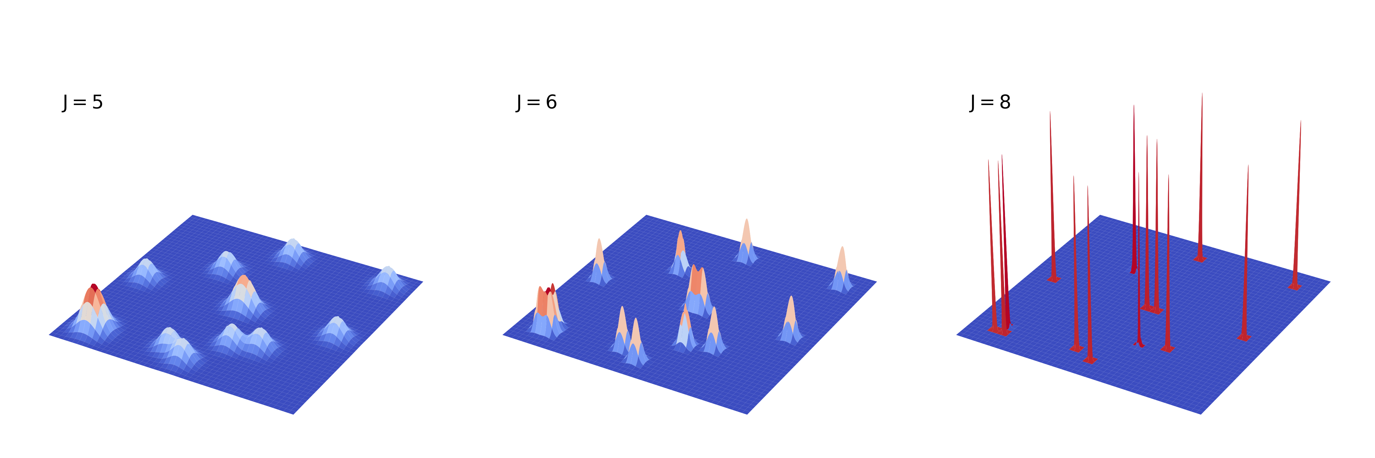
_images/hmFig0_delta.png — Multiresolution field reconstruction in the Hermes paper: a discrete catalogue is represented by compact scaling-function coefficients and may then be evaluated as a continuous field.#

Resolution and the role of J#

The MRA grid has

\[L = 2^J, \qquad N_{\mathrm{MRA}} = L^3 = 2^{3J}, \qquad \Delta x = \frac{L_{\mathrm{box}}}{2^J}.\]

Increasing J by one halves the nominal cell size and multiplies the number of three-dimensional coefficients by eight. The scaling functions are not nearest-grid-point cells, but \(\Delta x\) remains the useful first check: measurements at separations or bin widths comparable to it require a convergence test.

The visual \(J=7,8,9\) reconstruction comparison and practical resolution guidance are kept with the projection workflow in Build an SFCField.

Normalisation carried by SFCField#

Projection weights are divided according to weight_normalization:

raw: No division. The field integral is \(\sum_i w_i q_i\).
catalog: Divide by \(\sum_i w_i\). For an unweighted number field the field integral is one. This is the default for catalogue statistics.
field: Divide by \(\sum_i w_i q_i\), giving a unit-integral weighted field.

unit is accepted by high-level tasks as a request to convert each input field to unit integral. On an SFCField itself, use to_unit_weight() or with_normalization("unit").

field_mean_density(value_unit="grid") divides the field integral by L**3. value_unit="physical" divides by box_size**3. The same choice is available when evaluating the continuous field with field_density_at_pos.

Window projection and convolution#

Let \(W(\mathbf{x})\) be a translation-invariant window and \(\widehat W(\mathbf{k})\) its Fourier transform. Projection onto the same scaling-function space introduces the autocorrelation factor \(\widehat\Phi\), so the stored discrete kernel is schematically

\[K_W(\mathbf{k}) = \widehat W(\mathbf{k})\widehat\Phi(\mathbf{k}).\]

Applying a window is then

\[\epsilon_W = \operatorname{iFT} \left[\operatorname{FT}(\epsilon)K_W\right].\]

In Python this is simply:

filtered = field @ window

The output is another SFCField. Field addition and subtraction combine coefficient arrays; field multiplication forms a coefficient-space product:

delta = data - random
local_product = (delta @ bin_window) * delta
spatial_average = local_product.as_array().mean()

The scaling-function connection relations make these coefficient-space products the MRA representation of the spatial products used by Hermes estimators.

One-point statistics#

A smoothing window \(W_R\) gives a local field \(F_R = F * W_R\). Counting samples this continuous filtered field at uniform random positions. Histograms, moments, and one-point PDFs are ordinary post-processing of the returned samples.

The one-field second moment can also be written as

\[\sigma_W^2(R) = \left\langle \delta_W^2(\mathbf{x})\right\rangle, \qquad \delta_W = \delta * W_R.\]

Changing the window changes the statistic: sphere and gaussian are low-pass filters; cw, cws, and gdw are localised high-pass or band-pass filters.

Two-point statistics#

Let \(D\) and \(R\) denote consistently normalised data and random fields, and \(\Delta = D-R\). For a separation-binning window \(W_b\), PyHermes evaluates

\[\Delta DD[W_b] = \left\langle (\Delta_1 * W_b)\,\Delta_2\right\rangle, \qquad RR[W_b] = \left\langle (R_1 * W_b)\,R_2\right\rangle,\]

and returns

\[\xi[W_b] = \frac{\Delta DD[W_b]}{RR[W_b]}.\]

This is the field form of the Landy–Szalay combination. The task may also return dd, dr, rd, delta_dd, and rr separately.

The geometry resides in \(W_b\):

shell gives an isotropic separation;
thick_shell and gaussian_shell average over a finite radial range;
ring maps \((s,\mu)\) into transverse and line-of-sight offsets;
disk, cylshell, and cylinder define alternative anisotropic averages.

Additional window1 and window2 filters act on the two input vertices before the binning window is applied.

Standard three-point statistics#

Corr_3PCF performs a Monte Carlo translational and rotational average for a triangle with fixed \(r_{12}\), \(r_{13}\), and sampled included angle. Its three input vertices may have independent smoothing windows.

center="particle" uses catalogue objects as primary vertices. This is the dual-sphere construction in the paper. center="box_random" samples primary vertices uniformly in the volume, corresponding to the triplet-sphere construction. n_rot controls the random rotational average around each centre.

The connected three-point statistic is assembled from data and random field products. zeta is the connected 3PCF and Q is the reduced 3PCF,

\[Q = \frac{\zeta} {\xi_{12}\xi_{13}+\xi_{12}\xi_{23}+\xi_{13}\xi_{23}}.\]

3PCF multipoles#

The angular dependence of the 3PCF can be expanded as

\[\zeta(r_{12},r_{13},\mu) = \sum_{\ell}(2\ell+1)\, \zeta_\ell(r_{12},r_{13})P_\ell(\mu).\]

For a thin shell, the Fourier-space multipole window has the form

\[W_{r}^{\ell m}(\mathbf{k}) = 4\pi i^\ell j_\ell(2\pi kr)Y_\ell^m(\widehat{\mathbf{k}}).\]

Corr_3PCF_Multipole constructs the required window-filtered \((\ell,m)\) fields and contracts their local products. Only \(m\geq0\) fields are built explicitly; negative modes follow from spherical-harmonic conjugation symmetry.

The two radial supports are supplied by binning_window12 and binning_window13. Thin shells use the analytic spherical-Bessel response. General radial profiles use \(U_\ell(k)Y_\ell^m\) kernels, with numerical spherical-Hankel tabulation when no direct analytic higher-order response is available.

Weighted and derived physical fields#

Weights modify the field before projection; windows modify it afterwards. This separation makes marked and physical-field statistics natural:

\[F_q(\mathbf{x}) = \sum_i w_i^{\mathrm c}w_i^{\mathrm{opt}}m_iq_i \delta_{\mathrm D}^{3}(\mathbf{x}-\mathbf{x}_i).\]

Factorisable catalogue weights belong in catalog_weight or field_value. A separation-dependent factor may belong in a window. General non-separable pair weights do not preserve one translation-invariant convolution and require a decomposition or explicit correction.

Operator windows use the Fourier identities

\[\widehat{\partial_{\hat n}f}=i(\mathbf{k}\cdot\hat{\mathbf n})\hat f, \qquad \widehat{\nabla^2 f}=-k^2\hat f, \qquad \widehat{\nabla^{-2}f}=-\frac{1}{k^2}\hat f.\]

The inverse-Laplacian zero mode is set to zero, fixing the arbitrary additive constant of the potential. Cosmological prefactors are intentionally applied outside that mathematical operator, where coordinate and unit conventions are explicit.

Projection and repeated windows#

The finite scaling-function projection matters when operations are composed. A WindowFunc stores \(K_W\), not a bare \(\widehat W\). Therefore:

field @ W1 @ W2 applies two projected kernels;
W1 * W2 multiplies two already projected kernels point by point;
neither expression is, in general, identical to projecting the continuous product \(\widehat W_1\widehat W_2\) exactly once.

For a production composite window, the cleanest current route is to define the complete Fourier expression in one built-in or custom window and apply it once. W1 * W2 remains useful for exploratory projected-kernel composition and for testing separable constructions, provided this distinction is kept in mind. See Window reference for code and kernel-mode details.