Two-point correlation functions

Corr_2PCF evaluates products of filtered data and random fields over a sampled family of separation-binning windows. The same estimator handles isotropic, anisotropic, auto-, and cross-correlations.

The complete 2PCF notebook connects the task interface to low-level field–window operations and includes isotropic and redshift-space visualisations.

Isotropic 2PCF

The smallest configuration uses thin spherical shells:

Corr_2PCF:
   sfc_field: ./output/quijote8000_snap004_sfc.pkl
   random: uniform
   binning_window: shell
   sampling:
      s: {min: 0.0, max: 150.0, n: 31}
   products: [dd, dr, rd, xi]
   threads: 2
   fout_path: ./output/quijote8000_snap004_2pcf.pkl

random: uniform uses the analytic constant reference density. Supply an SFCField or path instead when the random catalogue is spatially varying.

Run and load:

cd examples
python scripts/run_2pcf.py configs/param_2pcf.yaml

from pyhermes.io import Corr2PCFData

corr = Corr2PCFData(
    data_path="./output/quijote8000_snap004_2pcf.pkl"
)
print(corr.sampling_names)  # ('s',)
print(corr.s, corr.xi)

Redshift-space anisotropy

A ring bin maps each \((s,\mu)\) sample to transverse radius \(R=s\sqrt{1-\mu^2}\) and line-of-sight offset \(H=s\mu\):

Corr_2PCF:
   sfc_field: ./output/quijote8000_snap004_rsd_sfc.pkl
   random: uniform
   binning_window: ring
   sampling:
      s: {min: 0.0, max: 180.0, n: 46}
      mu: {min: 0.0, max: 1.0, n: 51}
   products: xi
   threads: 8
   fout_path: ./output/quijote8000_snap004_rsd_2pcf_smu.pkl

The result has xi.shape == (len(s), len(mu)). The plotting helper converts it to the \((s_\perp,s_\parallel)\) plane:

from pyhermes.io import Corr2PCFData
from pyhermes.utils.plot import plot_corr2pcf_2d

corr_smu = Corr2PCFData(
    data_path="./output/quijote8000_snap004_rsd_2pcf_smu.pkl"
)
plot_corr2pcf_2d(corr_smu)

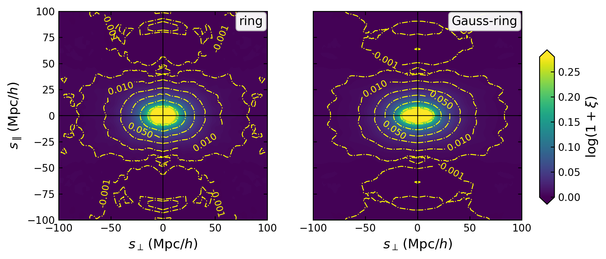
The same redshift-space estimator with a thin ring and a transversely Gaussian-blurred ring. The window changes; the field product does not.

Smoothing and binning are separate

Use window to smooth both vertices, or window1 and window2 for independent filters. Use binning_window for the pair separation:

Corr_2PCF:
   sfc_field: ./output/quijote8000_snap004_sfc.pkl
   random: uniform
   window:
      type: gaussian
      len_args: {R: 5.0}
   binning_window:
      type: thick_shell
      len_args:
         R: null
         delta_R: 6.0
      other_args: {}
      mapping: s_to_R
   sampling:
      s: {min: 10.0, max: 150.0, n: 29}
   products: xi

The named mapping fills R from s and preserves the fixed delta_R. For a non-standard parameter mapping, provide a Python callable; 2PCF mappings are either one of the named mappings or a callable, not a YAML dictionary. See Window reference for all built-in geometries.

Result products

products may request:

dd

Data–data field product.

dr and rd

Ordered data–random cross-products.

delta_dd

Product of \(\Delta=D-R\) fields.

rr

Random–random normalisation.

xi

delta_dd / rr. Dependencies are computed automatically.

Only requested products and their dependencies are retained in the result.

Cross-correlations

Use independent vertices for a cross-correlation:

from pyhermes.theory.corr2pcf import Corr_2PCF

task = Corr_2PCF()
task.sfc_field1 = halo_field
task.sfc_field2 = mass_field
task.random1 = "uniform"
task.random2 = "uniform"
task.window1 = {"type": "gaussian", "len_args": {"R": 5.0}}
task.window2 = {"type": "gaussian", "len_args": {"R": 10.0}}
task.binning_window = {
    "type": "shell",
    "len_args": {"R": None},
    "other_args": {},
    "mapping": "s_to_R",
}
task.sampling = {"s": [20.0, 40.0, 60.0, 80.0]}
task.products = ["xi"]
cross = task.run(save_result=False)

All field vertices must share the same MRA geometry and basis. Task-level weight_normalization converts compatible catalogue fields to one common normalisation before products are formed.

Python overrides

import numpy as np
import copy

from pyhermes.param.parambase import read_param
from pyhermes.theory.corr2pcf import Corr_2PCF

params = read_param(config_path="./configs/param_2pcf.yaml")

def s_to_gaussian_shell(sample, template):
    mapped = copy.deepcopy(template)
    mapped["len_args"]["R_shell"] = sample["s"]
    return mapped

task = Corr_2PCF(params)
task.sampling = {"s": np.linspace(0.0, 180.0, 46)}
task.binning_window = {
    "type": "gaussian_shell",
    "len_args": {"R_smooth": 5.0},
    "mapping": s_to_gaussian_shell,
}
task.products = ["xi"]
result = task.run(save_result=False)

Resolution and bin width

The smallest trustworthy scale is controlled jointly by field resolution and the binning window. A narrow bin does not recover structure unresolved by J; a broad bin can intentionally average small-scale variation.

The direct periodic pair-counting comparison and its \(J\) convergence are shown on Validation and Performance. Residual differences are concentrated where the separation approaches the field resolution.

Performance controls

Sampling points are distributed across MPI ranks. The dominant cost is one window construction and convolution per sampled bin and required product.

memory_strategy: speed keeps reusable fields in memory. memory reloads or rebuilds more aggressively to reduce peak storage. binning_window_cache can persist expensive kernels across repeated runs; set an explicit binning_window_cache_dir for production jobs.

Public tutorial

The rendered 2PCF notebook contains high- and low-level isotropic reconstruction, anisotropic window composition, saved RSD results, and custom ring tests. examples/scripts/run_2pcf.py is the production entry point.