Standard 3PCF

Corr_3PCF measures the angular three-point correlation function for a triangle with fixed sides \(r_{12}\) and \(r_{13}\). It evaluates the two displaced vertices as window-filtered fields, samples their product around a set of primary vertices, and averages over random rotations. This is the direct-angular counterpart of the harmonic estimator described in 3PCF multipoles.

The complete 3PCF notebook compares the two standard-3PCF centre strategies and shows how the saved count-level products assemble into \(\zeta\) and the reduced statistic \(Q\). Its later sections introduce the multipole estimator.

Triangle convention

The primary vertex is labelled 1. The two fixed sides are \(r_{12}=|\mathbf{x}_2-\mathbf{x}_1|\) and \(r_{13}=|\mathbf{x}_3-\mathbf{x}_1|\); the angular coordinate is either \(\theta\) or \(\mu=\cos\theta\). The third side follows from

\[r_{23}^2=r_{12}^2+r_{13}^2-2r_{12}r_{13}\mu.\]

For every angular sample, PyHermes rotates this triangle n_rot times. The rotation average is Monte Carlo: increasing n_rot reduces orientation noise but increases runtime approximately linearly.

A minimal run

The example configuration below uses halo positions as primary vertices and applies a \(5\,h^{-1}\mathrm{Mpc}\) spherical window to the displaced vertices:

Corr_3PCF:
   sfc_field: "./output/quijote8000_snap004_sfc.pkl"
   random: "uniform"
   window:
      type: "sphere"
      len_args:
         R: 5.0
   r12: 20.0
   r13: 40.0
   angle_param: "theta"
   theta:
      n_theta: 20
   n_rot: 20
   center: "particle"
   products: ["ddd", "Q"]
   base_seed: 42
   threads: 2
   fout_path: "./output/quijote8000_snap004_3pcf_pcenter_nrot20.pkl"

Run the tracked example from examples/:

python scripts/run_3pcf.py configs/param_3pcf_pcenter_nrot20.yaml

or construct the task directly:

from pyhermes.param.parambase import read_param
from pyhermes.theory import Corr_3PCF

params = read_param(config_path="./configs/param_3pcf_pcenter_nrot20.yaml")
result = Corr_3PCF(params).run()

Choosing primary vertices

center: particle

The first vertex is sampled at catalogue positions. This is efficient for sparse tracer catalogues and gives a dual-window estimator: window2 and window3 act on the two displaced vertices, while window1 has no effect on the naked particle centre. The input SFCField must retain companion particle data, or particle_pos1 and particle_weight1 must be passed together.

center: box_random

n_box_centers positions are drawn uniformly in the periodic box. All three vertices are evaluated as fields, so window1, window2, and window3 can all be active. This mode is useful for dense particle samples or whenever the primary field itself must be filtered.

The shared window is copied to every vertex that does not define an explicit window1, window2, or window3. In particle-centre mode this still does not filter the first vertex. Use explicit vertex windows when that distinction should be visible in the configuration.

For box-random centres, change only the centre section:

center: "box_random"
n_box_centers: 1000000
window2:
   type: "sphere"
   len_args: {R: 5.0}
window3:
   type: "sphere"
   len_args: {R: 5.0}

Data, randoms, and products

sfc_field supplies a shared data field; sfc_field1 through sfc_field3 override individual vertices. The random inputs follow the same pattern. random: uniform uses the analytic constant-density shortcut, whereas a path or SFCField represents an explicit random catalogue.

Requesting a final statistic automatically expands its dependencies:

Main standard-3PCF products

Product	Meaning
ddd, rrr	Raw data and random triplet products.
delta_ddd	Connected data-minus-random triplet combination.
xi12, xi13, xi23	Two-point terms on the three triangle sides.
zeta	Connected three-point correlation function.
zeta_H	Hierarchical denominator \(\xi_{12}\xi_{13}+\xi_{12}\xi_{23}+\xi_{13}\xi_{23}\).
Q	Reduced 3PCF, \(Q=\zeta/\zeta_H\).

The particle-centre mode additionally exposes d_delta_dd and r_delta_dd, the two centre-weighted contributions used to form delta_ddd. Product availability is validated against the selected centre mode; unsupported combinations fail early rather than silently changing the estimator.

Angle sampling

Set angle_param to theta or mu and configure the matching section:

angle_param: "mu"
mu:
   mu_min: -1.0
   mu_max: 1.0
   n_mu: 20

Explicit one-dimensional arrays are also accepted from Python. The output stores both theta and mu together with r23, so downstream plotting does not need to reconstruct the triangle geometry.

Reading a result

from pyhermes.io import Corr3PCFData

data = Corr3PCFData(
    data_path="./output/quijote8000_snap004_3pcf_pcenter_nrot20.pkl"
)
theta, Q = data.theta, data.Q

The arrays requested through products are available as attributes such as data.ddd, data.zeta, and data.Q. Configuration and field metadata are retained in data.corr3pcf_info and data.sfc_info1 through data.sfc_info3.

Connection to multipoles

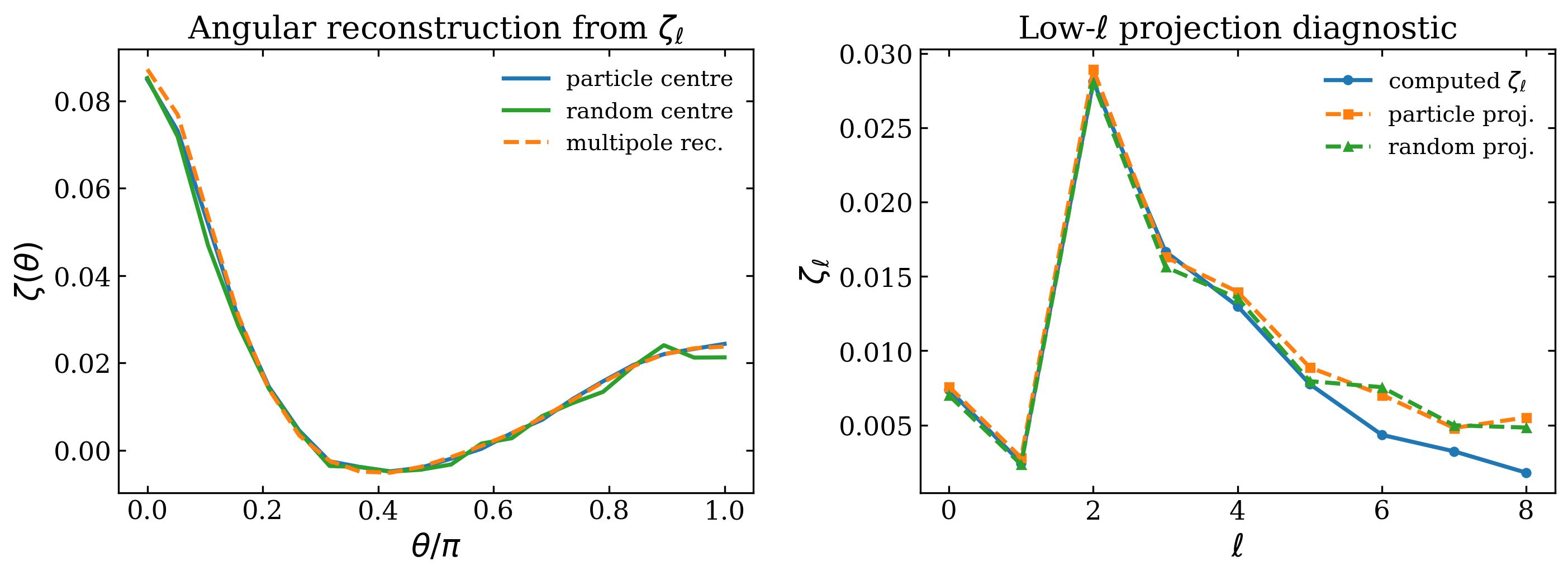
Direct angular estimates and the 3PCF multipole representation describe the same rotationally averaged signal. Residual differences arise from finite angular sampling, random rotations, centre sampling, and multipole truncation.

Use this task when the angular curve itself is the desired product. Use Corr_3PCF_Multipole when many angular configurations, high angular order, or radial-window scans are more naturally represented through \(\zeta_\ell\).