Physical fields from field–window operations

The field–window language is not limited to tracer counts. Catalogue weights and particle-carried values change what field is represented; windows change what operation is applied to that field. The same SFCProjection and WindowFunc objects can therefore construct velocity and momentum fields, differential operators, the Newtonian potential, acceleration, and marked density fields.

The executable Physical Fields notebook follows Build an SFCField and Field and window operations: projection defines the physical field, while windows apply smoothing and differential operators. The notebook keeps these calculations compact and spends most of its length on slice selection and publication-quality visualisation.

Catalogue weight versus field value

For particle positions \(\mathbf{x}_i\), PyHermes projects

\[F_q(\mathbf{x})= \sum_i {w_i^{\rm cat}q_i\over Z} \delta_{\rm D}^{(3)}(\mathbf{x}-\mathbf{x}_i).\]

catalog_weight holds completeness, selection, or other catalogue weights. field_value holds the quantity carried by each object: a mark, mass, or one velocity component. Keeping these roles separate prevents a signed physical quantity from being mistaken for a normalization weight.

weight_normalization chooses \(Z\):

• catalog divides by \(\sum_i w_i^{\rm cat}\) and is the default for normalized clustering fields.

• raw uses \(Z=1\); choose it when the absolute physical amplitude is required.

• field divides by \(\sum_i w_i^{\rm cat}q_i\) and is appropriate only when that field sum is meaningful and non-zero.

One small helper can build a family of fields on identical MRA metadata:

import numpy as np
from pyhermes.base.sfc_projection import SFCProjection

base = {
    "box_size": 1000.0,
    "J": 8,
    "wavelet_mode": "db2",
    "wavelet_level": 10,
    "phi_resolution": 1024,
    "threads": 8,
}

def project(pos, value=None, normalization="catalog"):
    params = dict(base, particle_pos=np.asarray(pos),
                  field_value=None if value is None else np.asarray(value),
                  weight_normalization=normalization)
    return SFCProjection({"SFCProjection": params}).run(save_result=False)

count = project(pos)
vx_weighted = project(pos, velocity[:, 0])

Velocity as a ratio of fields

A velocity-weighted field is not yet a volume-weighted velocity. After applying the same smoothing window to numerator and denominator,

\[v_i(\mathbf{x})={n_{v_i}(\mathbf{x})\over n(\mathbf{x})}.\]

The derivative must obey the quotient rule:

\[\partial_j v_i= {\partial_j n_{v_i}\over n} -{n_{v_i}\,\partial_j n\over n^2}.\]

This distinction matters in sparse regions. Mask points where the smoothed count field is too small instead of allowing a tiny denominator to manufacture large velocities.

Differential windows

With the package Fourier convention, a directional derivative along the unit vector \(\widehat{\mathbf n}\) is the multiplier

\[\widehat W_{\partial_{\widehat n}}(\mathbf{k}) =2\pi i(\mathbf{k}\cdot\widehat{\mathbf n}).\]

Three such windows give gradients; component combinations give divergence and curl. The Laplacian window applies \(-(2\pi k)^2\).

from pyhermes.io import WindowFunc

smooth = WindowFunc(
    {"type": "gaussian", "len_args": {"R": 10.0}},
    count.sfc_info,
    threads=8,
)
dx = WindowFunc(
    {
        "type": "directional_derivative",
        "los_args": {"nx": 1.0, "ny": 0.0, "nz": 0.0},
    },
    count.sfc_info,
    threads=8,
)

dcount_dx = count @ smooth @ dx

Window derivatives are formed in grid coordinates. Multiply sampled values by field.scale_factor when converting one derivative to inverse physical-box units. This is why the tutorial keeps coordinate conversion adjacent to the sampling code rather than hiding it inside the mathematical window.

Potential from the inverse Laplacian

The built-in inverse_laplacian is deliberately a pure mathematical operator:

\[\widehat W_{\nabla^{-2}}(\mathbf{k})= -{1\over(2\pi k)^2},\qquad \widehat W_{\nabla^{-2}}(0)=0.\]

Removing the zero mode fixes the arbitrary additive constant of the potential; it does not discard a measurable force. For the matter contrast \(\delta_{\rm m}\) in comoving coordinates,

\[{\Phi\over c^2} ={3\Omega_{\rm m0}H_0^2\over2ac^2} \nabla^{-2}\delta_{\rm m}.\]

Keeping the cosmological prefactor outside WindowFunc makes units and coordinate conventions explicit. If the box coordinates are in \(h^{-1}\mathrm{Mpc}\), use \(H_0=100\,\mathrm{km\,s^{-1}}/(h^{-1}\mathrm{Mpc})\); the numerical \(h\) is already carried by the coordinate unit. The notebook also multiplies the grid-space inverse Laplacian by the squared cell size.

inv_lap = WindowFunc(
    {"type": "inverse_laplacian"}, delta_m.sfc_info, threads=8
)
inv_lap_delta = delta_m @ inv_lap

c_light = 299792.458             # km/s
H0 = 100.0                       # km/s/(Mpc/h)
cell_size = delta_m.box_size / delta_m.L
poisson_scale = (
    1.5 * omega_m0 * (H0 / c_light) ** 2 / a * cell_size**2
)
phi_over_c2 = inv_lap_delta * poisson_scale

The resulting \(\Phi/c^2\) is dimensionless and mean-zero. Its broad, smooth appearance is physical: the \(k^{-2}\) response strongly emphasizes large scales.

Acceleration and linear flow

Directional derivatives of the potential give the peculiar acceleration,

\[\mathbf{g}=-{c^2\over a}\nabla_x(\Phi/c^2).\]

In linear theory the matter contrast, velocity divergence, potential, and acceleration are linked by the continuity and Poisson equations. After matching units and smoothing scales, their large-scale patterns should correlate; exact point-by-point equality is not expected for halo velocities because of bias, nonlinear motions, sparse sampling, and reconstruction error.

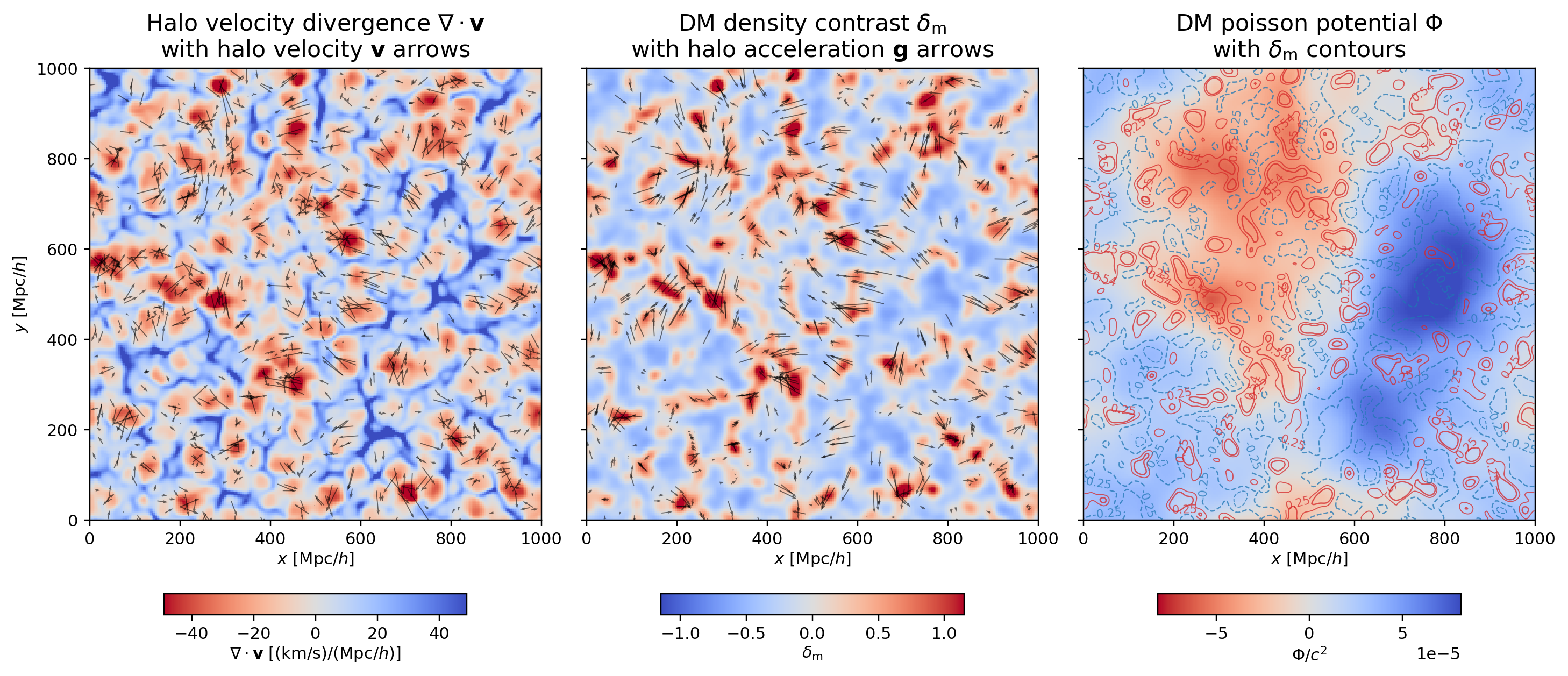
Halo velocity divergence, smoothed matter contrast, and the Newtonian potential on a common slice. Velocity and acceleration arrows expose the large-scale flow rather than merely the scalar amplitudes.

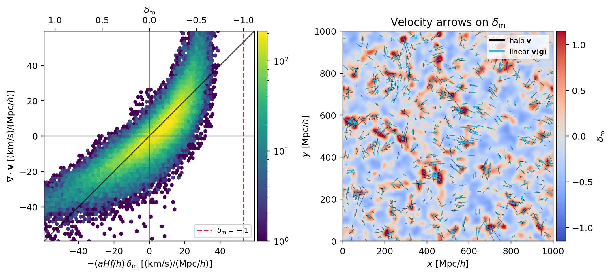
Linear-theory checks are most informative after using the same smoothing scale and evaluating both fields at matched positions.

Marked 2PCFs

A mark is simply another field_value. A common choice derives it from a local smoothed density, for example

\[m_{\rm power}=(\rho_R+\epsilon)^\alpha, \qquad m_{\rm inverse}=\left({\rho_*+1\over\rho_*+\rho_R}\right)^p.\]

Evaluate \(\rho_R\) at catalogue positions, normalize the marks by their catalogue-weighted mean, project the marked catalogue, and pass that SFCField to the unchanged Corr_2PCF task. No marked-pair estimator is needed: the mark changes the field, not the binning operation.

This is a direct extension of the same projection pattern rather than a cell in physical_fields.ipynb. The companion notebook concentrates on velocity, momentum, potential, and acceleration; continue with Two-point correlation functions when applying a projected mark to the 2PCF.

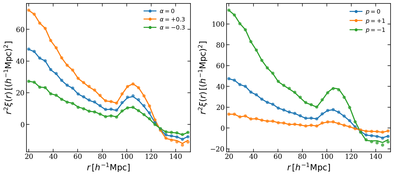
Power-law and inverse-density marks emphasize different environments while reusing the same 2PCF field–window estimator.

Scope and interpretation

These operator windows make many derived fields concise, but they do not make all of them automatically physical. Always state the catalogue normalization, coordinate units, smoothing scale, zero-mode convention, and whether the field is tracer- or matter-based. The algebra is short; the assumptions still deserve their full names.