Window reference#

WindowFunc is the common operator interface in PyHermes. A window may smooth a field, define a separation bin, select a multipole, or apply a mathematical operator. Its scientific role is determined by where the task uses it, not by a separate class hierarchy.

Basic construction#

Every window must be constructed with metadata from a compatible SFCField:

from pyhermes.io import SFCField, WindowFunc

D = SFCField(data_path="./output/quijote8000_snap004_sfc.pkl", threads=8)
W = WindowFunc(
    {"type": "gaussian", "len_args": {"R": 10.0}},
    D.sfc_info,
    threads=8,
)
D_smoothed = D @ W

The parameter dictionary has four main sections:

type: Name of a built-in window.
len_args: Physical length parameters in the same units as box_size. PyHermes rescales them to MRA-grid coordinates internally.
los_args: A line-of-sight direction nx, ny, nz. The default is the positive z axis.
other_args: Dimensionless or profile-specific controls.

Built-in ordinary windows#

The Fourier expressions below use angular wavenumber \(k\). Built-in functions are evaluated internally in cycle-frequency grid coordinates, where the required factors of \(2\pi\) are included by the implementation. Unit-integral smoothing and binning windows satisfy \(\widehat W(0)=1\).

Type	Role	Length arguments	Fourier response
`sphere`	Spherical top-hat	`R`	\(3[\sin(kR)-kR\cos(kR)]/(kR)^3\)
`gaussian`	Isotropic low-pass filter	`R`	\(\exp[-k^2R^2/2]\)
`shell`	Infinitesimal spherical bin	`R`	\(j_0(kR)=\sin(kR)/(kR)\)
`thick_shell`	Finite spherical bin	`R`, `delta_R`	Volume-weighted difference of two `sphere` responses
`gaussian_shell`	Smooth radial shell	`R_shell`, `R_smooth`	Gaussian-damped shell response
`cubic`	Axis-aligned box top-hat	`Lx`, `Ly`, `Lz`	Product of three sinc factors
`ring`	Thin anisotropic pair bin	`R`, `H`	\(J_0(k_\perp R)\cos(k_\parallel H)\)
`disk`	Filled transverse disk at \(\pm H\)	`R`, `H`	\(2J_1(k_\perp R)/(k_\perp R)\cos(k_\parallel H)\)
`cylshell`	Cylindrical side wall	`R`, `H`	\(J_0(k_\perp R)\operatorname{sinc}(k_\parallel H)\)
`cylinder`	Filled finite cylinder	`R`, `H`	Disk factor times line-of-sight sinc

For ring and disk, H is the line-of-sight offset. For cylshell and cylinder, H is the half-height, so the real-space support is \(|z|\leq H\).

thick_shell clips its inner radius at zero and requires delta_R > 0:

W_bin = WindowFunc(
    {
        "type": "thick_shell",
        "len_args": {"R": 40.0, "delta_R": 6.0},
    },
    D.sfc_info,
    threads=8,
)

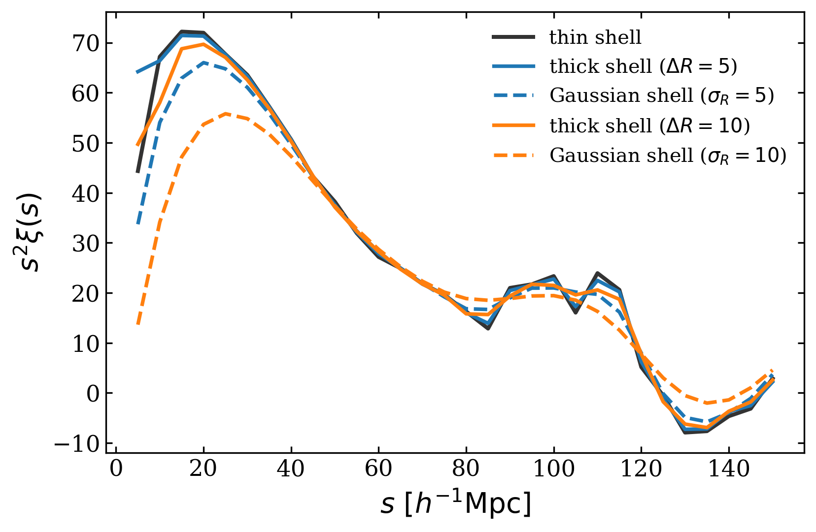
_images/corr2pcf_binning_window_shell_gaussian_shell_comparison.png — Thin, finite-thickness, and Gaussian-shell bins change the effective radial averaging while leaving the 2PCF estimator itself unchanged.#

High-pass and wavelet-like filters#

cw, cws, and gdw are scale-normalised, zero-mean filters used to isolate localised fluctuations and band-averaged power. They take len_args: {R: ...}.

cw: Cosine-wavelet response.
cws: Spherical cosine-wavelet response.
gdw: Isotropic Gaussian-derivative wavelet, proportional to \((kR)^2\exp[-(kR)^2/2]\) in Fourier space.

These filters do not satisfy \(\widehat W(0)=1\); their zero mode vanishes by design. Their amplitude is scale-normalised, so do not interpret them as ordinary local-density averages.

Differential and inverse operators#

Type	Parameters	Kernel
`directional_derivative`	`los_args: {nx, ny, nz}`	\(i\,\mathbf{k}\cdot\hat{\mathbf n}\)
`laplacian`	none	\(-k^2\)
`inverse_laplacian`	none	\(-1/k^2\), with the zero mode set to zero

In the code’s cycle-frequency convention the derivative includes \(2\pi\) and the Laplacian includes \((2\pi)^2\). Length rescaling by L / box_size is handled consistently with other windows.

Dx = WindowFunc(
    {
        "type": "directional_derivative",
        "los_args": {"nx": 1.0, "ny": 0.0, "nz": 0.0},
    },
    D.sfc_info,
    threads=8,
)
grad_x = D @ Dx

For a density contrast \(\delta_m\), inverse_laplacian returns \(\nabla^{-2}\delta_m\). Multiply by the physical Poisson prefactor outside the window, where the scale factor, Hubble convention, speed of light, and coordinate units are explicit.

Smoothing windows and binning windows#

The distinction is semantic and important:

a task window or window1/window2/window3 filters an input field vertex before the estimator is assembled;
a binning_window maps sampled coordinates into the spatial support of a pair or triangle edge.

For example, this 2PCF smooths both data vertices with a spherical top-hat and then samples thin-shell separations:

Corr_2PCF:
   sfc_field: ./output/halo_sfc.pkl
   random: uniform
   window:
      type: sphere
      len_args: {R: 5.0}
   binning_window: shell
   sampling:
      s: {min: 0.0, max: 150.0, n: 31}
   products: xi

Changing window changes the fields being correlated. Changing binning_window changes the definition of the sampled separation bin.

Line-of-sight geometry#

Axis-aligned LOS directions are:

los_args: {nx: 0.0, ny: 0.0, nz: 1.0}

For a ring 2PCF sampled in \((s,\mu)\), the built-in smu_to_RH mapping sets

\[R=s\sqrt{1-\mu^2}, \qquad H=s\mu.\]

The short YAML form applies this mapping automatically:

binning_window: ring
sampling:
   s: {min: 0.0, max: 180.0, n: 46}
   mu: {min: 0.0, max: 1.0, n: 51}

The explicit form is useful when setting the LOS or kernel mode:

binning_window:
   type: ring
   len_args: [R, H]
   mapping: smu_to_RH
   los_args: {nx: 0.0, ny: 0.0, nz: 1.0}
   kernel_mode: octant

2PCF sampling mappings#

Corr_2PCF provides three named mappings:

s_to_R: Set R = s for isotropic shell-like windows.
smu_to_RH: Set R = s*sqrt(1-mu**2) and H = s*mu.
rppi_to_RH: Set R = rp and H = pi.

Short string values such as binning_window: shell and binning_window: ring are normalised to the appropriate defaults by the task.

3PCF-multipole radial mappings#

Corr_3PCF_Multipole uses explicit mappings from sampled parameter names to the two edge windows:

binning_window12:
   type: thick_shell
   len_args: {delta_R: 6.0}
   mapping: {R: r12}
binning_window13:
   type: gaussian_shell
   len_args: {R_smooth: 6.0}
   mapping: {R_shell: r13}
sampling:
   mode: paired
   r12: 20.0
   r13: {start: 40.0, stop: 140.0, step: 5.0}

mode: grid forms the Cartesian product of all sampled arrays. mode: paired aligns arrays element by element; each array must have either one value or the common sample count.

Radial multipole profiles#

For 3PCF multipoles, an edge window becomes \(U_\ell(k)Y_\ell^m(\hat{\mathbf{k}})\).

shell uses the analytic \(j_\ell(kr)\) response at every order.
the monopoles of the other built-ins use their direct analytic Fourier responses;
higher orders for sphere, thick_shell, and gaussian are tabulated from analytic real-space profiles;
higher orders for gaussian_shell use the general inverse-Hankel route;
local cubic interpolation evaluates the resulting one-dimensional \(U_\ell(k)\) table while constructing the three-dimensional kernel.

The task can diagnose radial-table accuracy with radial_profile_diagnostics, radial_profile_diagnostic_tolerance, and radial_profile_diagnostic_probes.

Custom radial profiles are Python-level inputs. Use the helpers in pyhermes.utils.radial_profiles:

import numpy as np
from pyhermes.utils.radial_profiles import real_space_profile

def compensated_profile(r, R):
    return np.where(r < R, 1.0, -0.125)

profile = real_space_profile(
    compensated_profile,
    r_max=2.0,
    normalization="unit_integral",
    allow_signed=True,
)

Pass the resulting dictionary through the binning window’s other_args and use type: custom_real. tabulated_real_space_profile and kspace_profile provide the corresponding tabulated-real and inverse-Hankel k-space routes. Callable profiles are not serialisable YAML values, so define them in Python after reading a base configuration.

Custom ordinary Fourier windows#

A custom ordinary window is a Numba-compatible function receiving grid cycle-frequencies ki, kj, and kk followed by the values from len_args, los_args, and other_args:

import numpy as np
from numba import njit

from pyhermes.io import WindowFunc

@njit
def transverse_gaussian(ki, kj, kk, R):
    q2 = (2.0 * np.pi * R) ** 2 * (ki * ki + kj * kj)
    return np.exp(-0.5 * q2)

W_perp = WindowFunc(
    {"func": transverse_gaussian, "len_args": {"R": 5.0}},
    D.sfc_info,
    threads=8,
)

Define removable singularities and the zero mode explicitly. Put every physical length in len_args so it receives the same grid rescaling as a built-in window. If type is also supplied, the explicit func takes precedence even when that name matches a built-in window. In that case the type is retained as metadata, while built-in argument defaults and validation are not applied.

Window arithmetic and its projection caveat#

Windows support addition, subtraction, scalar multiplication and division, and pointwise multiplication:

R, delta_R = 40.0, 6.0
r_in = R - 0.5 * delta_R
r_out = R + 0.5 * delta_R

W_in = WindowFunc(
    {"type": "sphere", "len_args": {"R": r_in}}, D.sfc_info
)
W_out = WindowFunc(
    {"type": "sphere", "len_args": {"R": r_out}}, D.sfc_info
)
W_projected_shell = (
    r_out**3 * W_out - r_in**3 * W_in
) / (r_out**3 - r_in**3)

Arithmetic materialises a composite w_kernel. Crucially, each operand is already a projected MRA kernel \(K_W=\widehat W\widehat\Phi\). Thus W1 * W2 computes \(K_{W_1}K_{W_2}\), not a fresh single projection of \(\widehat W_1\widehat W_2\).

For exact control of one continuous composite expression, implement the full Fourier product in one custom function or use a built-in composite window such as thick_shell. Projected-kernel arithmetic is still useful for rapid experiments and for quantifying projection effects, but it should be named as such in an analysis.

Kernel modes#

kernel_mode controls how the discrete kernel is built:

octant: Build one real symmetric octant and fold it to an rFFT kernel. Fast and appropriate for even, axis-aligned real windows.
full_rfft: Evaluate every stored rFFT mode. Use it for a real window without octant symmetry, including an oblique LOS.
complex_rfft: Build a directional complex rFFT kernel, used by first derivatives.
complex_full_fft: Build a full complex FFT kernel, required by spherical-harmonic multipole windows.
auto: Select a compatible mode from the window type and LOS. Custom ordinary windows default conservatively to full_rfft.

octant and full_rfft evaluate the same projected real kernel when the symmetry assumptions hold. The difference is construction strategy, not a different physical window. An invalid symmetry assumption, however, can fold distinct modes together and change the result.

Practical checks#

Match J, box_size, wavelet_mode, wavelet_level, and phi_resolution between fields and windows.
Compare the MRA cell scale with every smoothing radius and bin width.
Treat smoothing parameters and binning parameters as part of the statistic’s definition and record them in plots and output names.
Use one complete custom kernel when composite-window accuracy matters.
Keep axis-aligned LOS choices when possible for cheaper kernel construction.
Enable binning-window caching only for repeated heavy runs where disk reuse outweighs cache management.