

Counting: Sample the Field at Random Positions#
This notebook continues from quick_start.ipynb and reuses its saved ./output/quijote8000_snap004_sfc.pkl. PyHermes turns that SFCField into a one-point sampling dataset: optionally smooth the field, evaluate it at many random positions, and study the resulting distribution.
The interpretation of the sampled values follows the upstream SFCField: a unit-value field samples a catalogue-normalized tracer density, while a mass-valued field carries the catalogue-weighted mean mass amplitude.
What this notebook emphasizes#
the standard task interfaces for
Countinghow
SFCFieldandWindowFuncare passed into the taskhow sampled values can be used to inspect the PDF of a smoothed tracer-density or mass-valued field
[1]:
from pyhermes.theory.counting import Counting
from pyhermes.param.parambase import read_param
from pyhermes.utils.sampling import random_box_positions
from pyhermes.io import WindowFunc, SFCField, CountingData
import matplotlib.pyplot as plt
import numpy as np

from pathlib import Path
import os
cwd = Path.cwd().resolve()
if cwd.name == "notebooks" and cwd.parent.name == "examples":
    examples_dir = cwd.parent
elif cwd.name == "examples":
    examples_dir = cwd
elif (cwd / "examples").is_dir():
    examples_dir = cwd / "examples"
else:
    raise RuntimeError("Run this notebook from the project root, examples/, or examples/notebooks/.")
os.chdir(examples_dir)
print(f"Working directory: {Path.cwd()}")

figs_dir = Path("figs")
figs_dir.mkdir(exist_ok=True)
Working directory: /Users/xutengpeng/xutp/PycharmProjects/PyHermes/examples
1. Standard Counting workflows#
All workflows below do the same conceptual job: draw random points in the box and evaluate either the unfiltered field or a smoothed version of it at those positions.
Minimal YAML Shapes#
Counting reads a saved SFCField field, optionally applies an ordinary smoothing window, and samples the result at random positions:
Counting:
   sfc_field: "./output/quijote8000_snap004_sfc.pkl"
   random_count: 10000000
   window:
      type: "sphere"
      len_args:
         R: 20
   threads: 8
   fout_path: "./output/quijote8000_snap004_counting_sph20.pkl"
Omit window if you want to sample the unfiltered field. When window is present, it is a normal smoothing WindowFunc, not a binning window.
Command-line entry point#
Use the standard driver when you want the cleanest path from config file to saved output.
[2]:
! python ./scripts/run_counting.py ./configs/param_counting.yaml
12:07:50 - INFO - pyhermes.param.parambase:ParamBase - Reading configure file: './configs/param_counting.yaml'
12:07:50 - INFO - pyhermes.param.parambase:ParamBase - Input parameter file format is YAML
12:07:50 - INFO - pyhermes.param.parambase:ParamBase - Set default parameters of module <theory> ...
12:07:50 - INFO - pyhermes.param.parambase:ParamBase - Default 'Counting.sfc_field' from 'empty' to './output/quijote8000_snap004_sfc.pkl'
12:07:50 - INFO - pyhermes.param.parambase:ParamBase - Default 'Counting.random_count' from '1000000' to '10000000'
12:07:50 - INFO - pyhermes.param.parambase:ParamBase - Default 'Counting.window.type' from 'empty' to 'sphere'
12:07:50 - WARNING - pyhermes.param.parambase:ParamBase - Adding non-default key: 'Counting.window.len_args.R'
12:07:50 - INFO - pyhermes.param.parambase:ParamBase - Default 'Counting.threads' from '1' to '8'
12:07:50 - INFO - pyhermes.param.parambase:ParamBase - Default 'Counting.fout_path' from 'empty' to './output/quijote8000_snap004_counting_sph20.pkl'

12:07:50 - INFO - pyhermes.pipeline.pipeline:Counting - Counting runtime configuration: running on 1 MPI ranks with 8 threads per rank
12:07:50 - INFO - pyhermes.pipeline.pipeline:Counting - Preparing Counting input field ...
12:07:50 - INFO - pyhermes.pipeline.pipeline:Counting - random_count=10000000, seed=42, threads=8
12:07:50 - INFO - pyhermes.io.base:SFCField - Reading SFCField data from ---> ./output/quijote8000_snap004_sfc.pkl <---
12:07:50 - INFO - pyhermes.io.base:SFCField - epsilon: Shape(256, 256, 256), Min = -3.215e-06, Max = 1.343e-05, Mean = 5.96e-08, Sum = 1
12:07:50 - INFO - pyhermes.pipeline.pipeline:Counting - Field weight normalization | field_kind=catalog_field | input=catalog | task=catalog | effective=catalog
12:07:51 - INFO - pyhermes.pipeline.pipeline:Counting - Counting field ready | source=path=./output/quijote8000_snap004_sfc.pkl | window=provided window dict | applying window type=sphere args={'R': 20}
12:07:51 - INFO - pyhermes.pipeline.pipeline:Counting - Start Counting ...
12:07:52 - INFO - pyhermes.pipeline.pipeline:Counting - Gathering data from all ranks ...
12:07:52 - INFO - pyhermes.pipeline.pipeline:Counting - The time for counting is: 1.0524 sec
12:07:52 - WARNING - pyhermes.io.funcs:check_fout - Output file './output/quijote8000_snap004_counting_sph20.pkl' already exists and will be overwritten (overwrite=True).
12:07:52 - INFO - pyhermes.io.base:CountingData - Writing Counting data to ---> ./output/quijote8000_snap004_counting_sph20.pkl <---

12:07:52 - INFO - pyhermes.pipeline.pipeline:Counting - The time for task: 2.5628 sec
Config-driven Python API#
This keeps the YAML config in control while making the resulting CountingData object immediately available in the notebook.
[3]:
counting_params = read_param('./configs/param_counting.yaml')
task = Counting(param_task=counting_params)
task.run(overwrite=True)
12:07:53 - INFO - pyhermes.param.parambase:ParamBase - Reading configure file: './configs/param_counting.yaml'
12:07:53 - INFO - pyhermes.param.parambase:ParamBase - Input parameter file format is YAML
12:07:53 - INFO - pyhermes.param.parambase:ParamBase - Set default parameters of module <theory> ...
12:07:53 - INFO - pyhermes.param.parambase:ParamBase - Default 'Counting.sfc_field' from 'empty' to './output/quijote8000_snap004_sfc.pkl'
12:07:53 - INFO - pyhermes.param.parambase:ParamBase - Default 'Counting.random_count' from '1000000' to '10000000'
12:07:53 - INFO - pyhermes.param.parambase:ParamBase - Default 'Counting.window.type' from 'empty' to 'sphere'
12:07:53 - WARNING - pyhermes.param.parambase:ParamBase - Adding non-default key: 'Counting.window.len_args.R'
12:07:53 - INFO - pyhermes.param.parambase:ParamBase - Default 'Counting.threads' from '1' to '8'
12:07:53 - INFO - pyhermes.param.parambase:ParamBase - Default 'Counting.fout_path' from 'empty' to './output/quijote8000_snap004_counting_sph20.pkl'

12:07:53 - INFO - pyhermes.pipeline.pipeline:Counting - Counting runtime configuration: running on 1 MPI ranks with 8 threads per rank
12:07:53 - INFO - pyhermes.pipeline.pipeline:Counting - Preparing Counting input field ...
12:07:53 - INFO - pyhermes.pipeline.pipeline:Counting - random_count=10000000, seed=42, threads=8
12:07:53 - INFO - pyhermes.io.base:SFCField - Reading SFCField data from ---> ./output/quijote8000_snap004_sfc.pkl <---
12:07:53 - INFO - pyhermes.io.base:SFCField - epsilon: Shape(256, 256, 256), Min = -3.215e-06, Max = 1.343e-05, Mean = 5.96e-08, Sum = 1
12:07:53 - INFO - pyhermes.pipeline.pipeline:Counting - Field weight normalization | field_kind=catalog_field | input=catalog | task=catalog | effective=catalog
12:07:54 - INFO - pyhermes.pipeline.pipeline:Counting - Counting field ready | source=path=./output/quijote8000_snap004_sfc.pkl | window=provided window dict | applying window type=sphere args={'R': 20}
12:07:54 - INFO - pyhermes.pipeline.pipeline:Counting - Start Counting ...
12:07:56 - INFO - pyhermes.pipeline.pipeline:Counting - Gathering data from all ranks ...
12:07:56 - INFO - pyhermes.pipeline.pipeline:Counting - The time for counting is: 1.2059 sec
12:07:56 - WARNING - pyhermes.io.funcs:check_fout - Output file './output/quijote8000_snap004_counting_sph20.pkl' already exists and will be overwritten (overwrite=True).
12:07:56 - INFO - pyhermes.io.base:CountingData - Writing Counting data to ---> ./output/quijote8000_snap004_counting_sph20.pkl <---

12:07:56 - INFO - pyhermes.pipeline.pipeline:Counting - The time for task: 3.0306 sec
[3]:
<pyhermes.io.counting.CountingData at 0x142ae8e00>
Task object overrides#
This version creates the task first and then adjusts a few attributes in Python. It is useful when you want to change the sample count, smoothing window, or threading without editing the config file.
Here the input is quijote8000_snap004_sfc_massweight.pkl, so counting_massw.nx samples a smoothed mass-valued field on the same catalogue measure rather than the unit-value tracer field.
[4]:
task = Counting()
task.threads = 8
task.random_count = 1000000
task.sfc_field = './output/quijote8000_snap004_sfc_massweight.pkl'
task.window = {"type": "sphere", "len_args": {"R": 20}}
counting_massw = task.run(save_result=False)
12:07:56 - INFO - pyhermes.param.parambase:ParamBase - Set default parameters of module <theory> ...

12:07:56 - INFO - pyhermes.pipeline.pipeline:Counting - Counting runtime configuration: running on 1 MPI ranks with 8 threads per rank
12:07:56 - INFO - pyhermes.pipeline.pipeline:Counting - Preparing Counting input field ...
12:07:56 - INFO - pyhermes.pipeline.pipeline:Counting - random_count=1000000, seed=42, threads=8
12:07:56 - INFO - pyhermes.io.base:SFCField - Reading SFCField data from ---> ./output/quijote8000_snap004_sfc_massweight.pkl <---
12:07:56 - INFO - pyhermes.io.base:SFCField - epsilon: Shape(256, 256, 256), Min = -2.705e+09, Max = 1.175e+10, Mean = 2.879e+06, Sum = 4.83e+13
12:07:56 - INFO - pyhermes.pipeline.pipeline:Counting - Field weight normalization | field_kind=catalog_field | input=catalog | task=catalog | effective=catalog
12:07:56 - INFO - pyhermes.pipeline.pipeline:Counting - Counting field ready | source=path=./output/quijote8000_snap004_sfc_massweight.pkl | window=provided window dict | applying window type=sphere args={'R': 20}
12:07:56 - INFO - pyhermes.pipeline.pipeline:Counting - Start Counting ...
12:07:56 - INFO - pyhermes.pipeline.pipeline:Counting - Gathering data from all ranks ...
12:07:56 - INFO - pyhermes.pipeline.pipeline:Counting - The time for counting is: 0.0735 sec

12:07:56 - INFO - pyhermes.pipeline.pipeline:Counting - The time for task: 0.4838 sec
Manual object preparation#
Here the upstream SFCField object and the smoothing window are created explicitly before they are passed into Counting. This makes the data flow fully visible.
[5]:
D = SFCField(data_path='./output/quijote8000_snap004_rsd_sfc.pkl', threads=8)
win_params = {"type": "sphere", "len_args": {"R": 20}}
filter_sph20 = WindowFunc(win_params, D.sfc_info, threads=8)

task = Counting()
task.threads = 8
task.random_count = 1000000
task.sfc_field = D.copy()
task.window = filter_sph20
counting_rsd = task.run(save_result=False)
12:07:56 - INFO - pyhermes.io.base:SFCField - Reading SFCField data from ---> ./output/quijote8000_snap004_rsd_sfc.pkl <---
12:07:56 - INFO - pyhermes.io.base:SFCField - epsilon: Shape(256, 256, 256), Min = -3.522e-06, Max = 1.761e-05, Mean = 5.96e-08, Sum = 1
12:07:56 - INFO - pyhermes.param.parambase:ParamBase - Set default parameters of module <theory> ...

12:07:57 - INFO - pyhermes.pipeline.pipeline:Counting - Counting runtime configuration: running on 1 MPI ranks with 8 threads per rank
12:07:57 - INFO - pyhermes.pipeline.pipeline:Counting - Preparing Counting input field ...
12:07:57 - INFO - pyhermes.pipeline.pipeline:Counting - random_count=1000000, seed=42, threads=8
12:07:57 - INFO - pyhermes.pipeline.pipeline:Counting - Field weight normalization | field_kind=catalog_field | input=catalog | task=catalog | effective=catalog
12:07:57 - INFO - pyhermes.pipeline.pipeline:Counting - Counting field ready | source=provided sfc_field | window=provided WindowFunc instance
12:07:57 - INFO - pyhermes.pipeline.pipeline:Counting - Start Counting ...
12:07:57 - INFO - pyhermes.pipeline.pipeline:Counting - Gathering data from all ranks ...
12:07:57 - INFO - pyhermes.pipeline.pipeline:Counting - The time for counting is: 0.0728 sec

12:07:57 - INFO - pyhermes.pipeline.pipeline:Counting - The time for task: 0.3616 sec
2. Inspect the saved counting result#
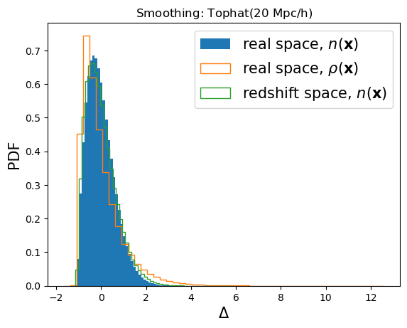
The saved CountingData object stores the sampled values. A histogram of counting.nx gives a quick view of the one-point distribution produced by the chosen smoothing scale.
The plot below normalizes each sampled field by its own mean. The unit-value real-space and redshift-space fields are shown as \(D(x) / \bar D - 1\), while the mass-valued run is shown after division by its catalogue-weighted mean mark. This keeps the contrast notation consistent while making clear which physical field was sampled.
[6]:
# read counting
counting_real = CountingData(data_path="./output/quijote8000_snap004_counting_sph20.pkl")

plt.hist(counting_real.nx/counting_real.nx.mean()-1, bins=50, density=True, label=r'real space, $n(\mathbf{x})$')
plt.hist(counting_massw.nx/counting_massw.nx.mean()-1, bins=50, density=True, histtype="step", label=r'real space, $\rho(\mathbf{x})$')
plt.hist(counting_rsd.nx/counting_rsd.nx.mean()-1, bins=50, density=True, histtype="step", label=r'redshift space, $n(\mathbf{x})$')
plt.legend(fontsize=15)
plt.title(r"Smoothing: Tophat(20 $\rm{Mpc}/h$)")
plt.xlabel(r'$\Delta$', fontsize=15)
plt.ylabel('PDF', fontsize=15)
plt.savefig(figs_dir / "counting_density_mass_rsd_pdf.png", dpi=200, bbox_inches="tight")
plt.show()
12:07:57 - INFO - pyhermes.io.base:CountingData - Reading Counting data from ---> ./output/quijote8000_snap004_counting_sph20.pkl <---
12:07:57 - INFO - pyhermes.io.base:CountingData - nx: Shape(10000000,), Min = -3.091e-10, Max = 5.407e-09, Mean = 1e-09
3. Low-level view: sample the smoothed field directly#
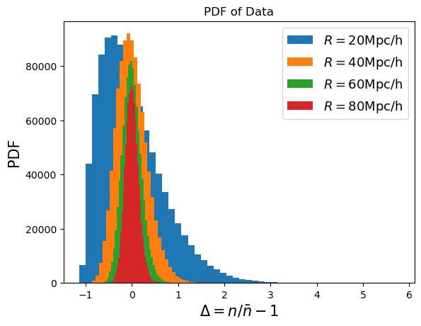
The cells below expose the same logic that the high-level Counting task uses internally. We first draw random positions in the simulation box, convolve the saved SFCField field with a chosen smoothing window, and evaluate the smoothed number density at those positions with field_density_at_pos.
For the unit-value halo field, the sampled values form a catalogue-normalized density. We convert them to density contrast using its known global mean, not the mean of the random sample,
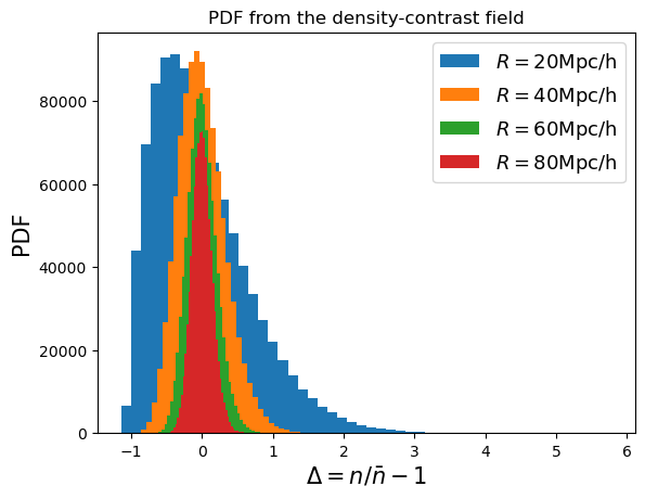
Equivalently, we can first build the full density-contrast field
then convolve and sample this derived field. With field_density_at_pos, derived fields use value_unit="grid" automatically, so a dimensionless density contrast is not rescaled as a catalogue density field. The two routes represent the same continuum operation; any remaining differences are numerical interpolation or finite-grid effects.
[7]:
rand = random_box_positions(10**6, D.box_size, seed=42)
win_params = dict(type="sphere", len_args={})
for smooth_radius in [20, 40, 60, 80]:
    win_params["len_args"]["R"] = smooth_radius
    filter = WindowFunc(win_params, D.sfc_info, threads=8)
    n = (D @ filter).field_density_at_pos(rand, value_unit="grid")
    delta_n = n / D.field_mean_density(value_unit="grid") - 1.0
    plt.hist(delta_n, bins=50, density=False, label=rf'$R={smooth_radius}$Mpc/h')

plt.title('PDF of Data')
plt.xlabel(r'$\Delta=n/{\bar n}-1$', fontsize=15)
plt.ylabel('PDF', fontsize=15)
plt.legend(fontsize=13)
plt.savefig(figs_dir / "counting_smoothing_radius_pdf.png", dpi=200, bbox_inches="tight")
plt.show()
[8]:
delta = D / D.field_mean_density(value_unit="grid") - 1.0
for smooth_radius in [20, 40, 60, 80]:
    win_params["len_args"]["R"] = smooth_radius
    filter = WindowFunc(win_params, D.sfc_info, threads=8)
    delta_n = (delta @ filter).field_density_at_pos(rand)
    plt.hist(delta_n, bins=50, density=False, label=rf'$R={smooth_radius}$Mpc/h')

plt.title(r'PDF from the density-contrast field')
plt.xlabel(r'$\Delta=n/{\bar n}-1$', fontsize=15)
plt.ylabel('PDF', fontsize=15)
plt.legend(fontsize=13)
plt.savefig(figs_dir / "counting_delta_field_smoothing_radius_pdf.png", dpi=200, bbox_inches="tight")
plt.show()
4. One-field second moment: \(\sigma_W(R)\)#
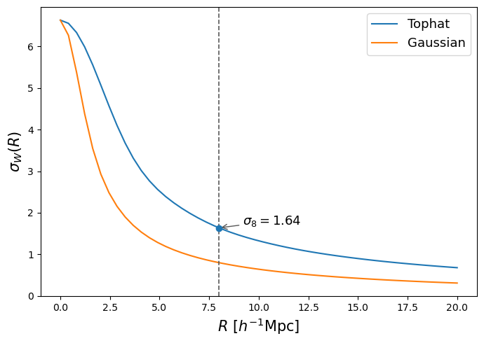
Once the density-contrast field is available, its smoothed one-point RMS fluctuation can be computed directly with PyHermes field algebra:
The helper compute_sigma_w below wraps this operation: build the requested window, convolve the density-contrast field, and return the RMS of the smoothed field. The first figure compares two low-pass smoothing families, spherical top-hat and Gaussian. The vertical dashed line marks \(R=8\,h^{-1}{\rm Mpc}\). In the standard cosmological convention, \(\sigma_8\) refers to the spherical top-hat RMS at this radius, so the marker is placed on the top-hat curve and its value is computed
directly at \(R=8\) rather than interpolated from the plotted sampling points. Here the plotted value is the corresponding RMS of the current halo density-contrast field, not the linear-theory matter \(\sigma_8\) parameter.
[9]:
def compute_sigma_w(delta_field, window_type, radius, *, threads=8):
    window = WindowFunc(
        {'type': window_type, 'len_args': {'R': float(radius)}},
        delta_field.sfc_info,
        threads=threads,
    )
    delta_w = delta_field @ window
    return np.sqrt((delta_w * delta_w).as_array().mean())


radii = np.linspace(0.0, 20.0, 50)
sigma_tophat = [compute_sigma_w(delta, 'sphere', radius) for radius in radii]
sigma_gauss = [compute_sigma_w(delta, 'gaussian', radius) for radius in radii]
sigma8 = compute_sigma_w(delta, 'sphere', 8.0)

plt.figure(figsize=(7, 5))
plt.plot(radii, sigma_tophat, label='Tophat')
plt.plot(radii, sigma_gauss, label='Gaussian')
plt.axvline(8.0, color='0.35', linestyle='--', linewidth=1.2)
plt.scatter([8.0], [sigma8], color='tab:blue', zorder=5)
plt.annotate(
    rf'$\sigma_8={sigma8:.3g}$',
    xy=(8.0, sigma8),
    xytext=(9.2, sigma8 * 1.05),
    arrowprops=dict(arrowstyle='->', color='0.35', lw=1.0),
    fontsize=13,
)
plt.xlabel(r'$R\ [h^{-1}{\rm Mpc}]$', fontsize=15)
plt.ylabel(r'$\sigma_W(R)$', fontsize=15)
plt.legend(fontsize=13)
plt.tight_layout()
plt.savefig(figs_dir / 'counting_sigma_lowpass.png', dpi=200, bbox_inches='tight')
plt.show()
High-pass response#
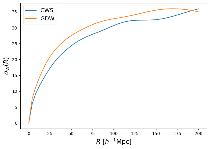
The same RMS definition can also be applied to high-pass or band-pass windows. Here we compare CWS, the three-dimensional spherical cosine wavelet, with GDW, the Gaussian-derivative wavelet. Both windows have vanishing response to the constant background, so the measured \(\sigma_W(R)\) reflects the scale-dependent fluctuation amplitude selected by the window rather than the large-scale mean density. Because CWS and GDW use different response shapes and normalizations, this figure is best read as a comparison of how the two high-pass kernels weight structure as their characteristic scale \(R\) changes.
[10]:
radii_hp = np.linspace(0.0, 200.0, 50)
sigma_cws = [compute_sigma_w(delta, 'cws', radius) for radius in radii_hp]
sigma_gdw = [compute_sigma_w(delta, 'gdw', radius) for radius in radii_hp]

plt.figure(figsize=(7, 5))
plt.plot(radii_hp, sigma_cws, label='CWS')
plt.plot(radii_hp, sigma_gdw, label='GDW')
plt.xlabel(r'$R\ [h^{-1}{\rm Mpc}]$', fontsize=15)
plt.ylabel(r'$\sigma_W(R)$', fontsize=15)
plt.legend(fontsize=13)
plt.tight_layout()
plt.savefig(figs_dir / 'counting_sigma_highpass.png', dpi=200, bbox_inches='tight')
plt.show()
Next steps#
Counting is the one-point-statistics branch of the example map. Continue with corr2pcf.ipynb for pair statistics and corr3pcf.ipynb for triangle statistics, or return to physical_fields.ipynb for differential operators acting on weighted physical fields.