

Window Functions and Field Algebra#
This notebook continues from the base field written by quick_start.ipynb and sits between projection and the measurement notebooks. After a catalog has been converted into a SFCField object, PyHermes lets you manipulate two objects directly:
SFCField: a multiresolution field, stored inepsilon.WindowFunc: a Fourier-space filter, stored asw_kernelafter it is built.
The goal here is to show the arithmetic supported by both objects, then introduce ordinary smoothing windows. These are not 2PCF binning_window definitions; binning windows are discussed in corr2pcf.ipynb.
[1]:
from pathlib import Path
import copy
import os

import numpy as np
from numba import njit

from pyhermes.io import SFCField, WindowFunc
from pyhermes.utils.special_functions import jn_numba
from pyhermes.utils.window_functions import (
    window_function_cylshell_numba,
    window_function_disk_numba,
    window_function_sphere_numba,
)

cwd = Path.cwd().resolve()
if cwd.name == "notebooks":
    os.chdir(cwd.parent)
elif (cwd / "examples").is_dir():
    os.chdir(cwd / "examples")

print(f"Working directory: {Path.cwd()}")
Working directory: /Users/xutengpeng/xutp/PycharmProjects/PyHermes/examples
1. Load Example Fields#
Quick Start builds D; sfc_projection.ipynb builds the explicit sampled random field R as part of its complete example field set. R is not required by the basic statistics tutorials, which can use the analytic uniform reference. Here both fields retain their raw total weights. To reproduce correlation-estimator algebra, we convert them to unit-total-weight fields; the scalar rho = 1 / V is the matching uniform-random shortcut.
[2]:
D = SFCField(data_path="./output/quijote8000_snap004_sfc.pkl", threads=8)
R = SFCField(data_path="./output/random_sfc.pkl", threads=8)

D_stat = D
R_stat = R
rho = 1.0 / D_stat.V
print(f"D.epsilon shape = {D.epsilon.shape}")
print(f"uniform density rho = {rho:.6e}")
11:37:57 - INFO - pyhermes.io.base:SFCField - Reading SFCField data from ---> ./output/quijote8000_snap004_sfc.pkl <---
11:37:57 - INFO - pyhermes.io.base:SFCField - epsilon: Shape(256, 256, 256), Min = -3.215e-06, Max = 1.343e-05, Mean = 5.96e-08, Sum = 1
11:37:57 - INFO - pyhermes.io.base:SFCField - Reading SFCField data from ---> ./output/random_sfc.pkl <---
11:37:58 - INFO - pyhermes.io.base:SFCField - epsilon: Shape(256, 256, 256), Min = -2.192e-07, Max = 9.48e-07, Mean = 5.96e-08, Sum = 1
D.epsilon shape = (256, 256, 256)
uniform density rho = 5.960464e-08
2. SFCField Arithmetic#
SFCField arithmetic acts on epsilon and returns a new SFCField object. This is useful for building density contrasts or simple derived fields before applying a window.
[3]:
delta_from_random = D_stat - R_stat
delta_from_uniform = D_stat - rho
mean_field = (D + R) / 2.0
scaled_delta = 2.0 * delta_from_uniform
field_product = D * R

print(delta_from_random.epsilon.shape)
print(mean_field.epsilon.shape)
print(scaled_delta.epsilon.shape)
print(field_product.epsilon.shape)
(256, 256, 256)
(256, 256, 256)
(256, 256, 256)
(256, 256, 256)
Supported field operations are:
D1 + D2
D1 - D2
D1 * D2
D + a
D - a
a - D
a * D
D * a
D / a
Here a is a scalar. Division is only defined as D / a; a / D and D1 / D2 are intentionally left out because their numerical and physical meaning is less clean.
3. Basic Smoothing with WindowFunc#
A WindowFunc is built from a small dictionary and the sfc_info of the field it will filter. The actual kernel is built lazily when the window is used by D @ W or when W.as_array() is called.
[4]:
def make_window(params, base=D):
    return WindowFunc(copy.deepcopy(params), base.sfc_info, threads=8)

W_sphere20 = make_window({"type": "sphere", "len_args": {"R": 20.0}})
D_sphere20 = D @ W_sphere20
delta_sphere20 = delta_from_uniform @ W_sphere20

print(D_sphere20.epsilon.shape)
print(delta_sphere20.epsilon.shape)
(256, 256, 256)
(256, 256, 256)
4. WindowFunc Arithmetic#
WindowFunc arithmetic acts on the materialized w_kernel. A composite window stores the combined kernel directly instead of trying to reconstruct a new Numba function. In particular, W1 * W2 is a projected-kernel product: it builds a composite window with W1.as_array() * W2.as_array(). This is useful when you want D @ (W1 * W2) to match (D @ W1) @ W2 up to FFT roundoff. It is not the same as multiplying two raw analytic transfer functions and projecting the product once.
[5]:
W_gauss8 = make_window({"type": "gaussian", "len_args": {"R": 8.0}})
W_mix = 0.7 * W_sphere20 + 0.3 * W_gauss8
W_chain = W_sphere20 * W_gauss8
D_mix = D @ W_mix
Supported window operations are:
W1 + W2
W1 - W2
W1 * W2
a * W
W * a
W / a
-W
Both windows in W1 + W2, W1 - W2, or W1 * W2 must be built for the same grid: the same J, box_size, phi_resolution, wavelet_mode, wavelet_level, bandwidth, and kernel shape. Write D @ (W1 * W2) when you want one convolution with the combined projected kernel.
5. Built-In Ordinary Windows#
The dictionaries below are ordinary smoothing/filter windows. They can be used as window, window1, window2, or a direct WindowFunc input. They are not yet 2PCF binning_window settings.
[6]:
builtin_window_params = {
    "sphere": {
        "type": "sphere",
        "len_args": {"R": 20.0},
    },
    "gaussian": {
        "type": "gaussian",
        "len_args": {"R": 8.0},
    },
    "shell": {
        "type": "shell",
        "len_args": {"R": 20.0},
    },
    "cubic": {
        "type": "cubic",
        "len_args": {"Lx": 20.0, "Ly": 20.0, "Lz": 20.0},
    },
    "ring": {
        "type": "ring",
        "len_args": {"R": 20.0, "H": 10.0},
        "los_args": [0.0, 0.0, 1.0],
    },
    "disk": {
        "type": "disk",
        "len_args": {"R": 20.0, "H": 10.0},
        "los_args": [0.0, 0.0, 1.0],
    },
    "cylshell": {
        "type": "cylshell",
        "len_args": {"R": 20.0, "H": 10.0},
        "los_args": [0.0, 0.0, 1.0],
    },
    "cylinder": {
        "type": "cylinder",
        "len_args": {"R": 20.0, "H": 10.0},
        "los_args": [0.0, 0.0, 1.0],
    },
}

for name, params in builtin_window_params.items():
    print(f"{name:9s}: {params}")
sphere   : {'type': 'sphere', 'len_args': {'R': 20.0}}
gaussian : {'type': 'gaussian', 'len_args': {'R': 8.0}}
shell    : {'type': 'shell', 'len_args': {'R': 20.0}}
cubic    : {'type': 'cubic', 'len_args': {'Lx': 20.0, 'Ly': 20.0, 'Lz': 20.0}}
ring     : {'type': 'ring', 'len_args': {'R': 20.0, 'H': 10.0}, 'los_args': [0.0, 0.0, 1.0]}
disk     : {'type': 'disk', 'len_args': {'R': 20.0, 'H': 10.0}, 'los_args': [0.0, 0.0, 1.0]}
cylshell : {'type': 'cylshell', 'len_args': {'R': 20.0, 'H': 10.0}, 'los_args': [0.0, 0.0, 1.0]}
cylinder : {'type': 'cylinder', 'len_args': {'R': 20.0, 'H': 10.0}, 'los_args': [0.0, 0.0, 1.0]}
[7]:
W_cubic20 = make_window(builtin_window_params["cubic"])
D_cubic20 = D @ W_cubic20
print(D_cubic20.epsilon.shape)
(256, 256, 256)
The line-of-sight windows (ring, disk, cylshell, cylinder) use los_args. Here H is a distance along the line of sight; for cylshell and cylinder, H is the half-height of the finite cylinder.
6. A Minimal Custom Window#
A custom window is a Numba function for the Fourier-space kernel. The first three arguments must be ki, kj, and kk. Length parameters go in len_args; dimensionless controls go in other_args; line-of-sight components go in los_args.
When both type and func are present, func defines the window even if type matches a built-in name. The type remains a useful label, but built-in argument defaults and validation are not applied.
[8]:
@njit
def window_function_cos_shell_numba(ki, kj, kk, R, amplitude=1.0):
    k = np.sqrt(ki * ki + kj * kj + kk * kk)
    q = 2.0 * np.pi * k * R
    return amplitude * np.cos(q)

cos_shell_params = {
    "type": "cos_shell",
    "func": window_function_cos_shell_numba,
    "len_args": {"R": 20.0},
    "other_args": {"amplitude": 1.0},
    "kernel_mode": "octant",
}

W_cos_shell = make_window(cos_shell_params)
D_cos_shell = D @ W_cos_shell
print(D_cos_shell.epsilon.shape)
(256, 256, 256)
kernel_mode="octant" is fast and works when the kernel is invariant under independent sign flips of kx, ky, and kz. For a general custom window, use kernel_mode="full_rfft"; for line-of-sight windows you can often use kernel_mode="auto".
7. Compose Windows from Built-In Pieces#
Composite windows are often easier to build from existing windows than to write from scratch. Linear combinations act directly on projected kernels and can reproduce linear formulas exactly. Products also act on projected kernels; they are useful for composing already projected convolution operators, while a raw analytic product would need a separate construction.
7.1 Finite-Thickness Spherical Shell#
A finite shell between R_in and R_out is a volume-weighted difference of two spherical top-hats:
W = (R_out**3 * W_sphere(R_out) - R_in**3 * W_sphere(R_in)) / (R_out**3 - R_in**3)
[9]:
@njit
def window_function_thick_shell_numba(ki, kj, kk, R_in, R_out):
    V_in = R_in**3
    V_out = R_out**3
    denom = V_out - V_in
    if denom == 0.0:
        k = np.sqrt(ki**2 + kj**2 + kk**2)
        q_out = 2.0 * np.pi * k * R_out
        if q_out == 0.0:
            return 1.0
        return np.sin(q_out) / q_out

    W_in = window_function_sphere_numba(ki, kj, kk, R_in)
    W_out = window_function_sphere_numba(ki, kj, kk, R_out)
    return (W_out * V_out - W_in * V_in) / denom
[10]:
R_in, R_out = 10.0, 20.0
W_inner = make_window({"type": "sphere", "len_args": {"R": R_in}})
W_outer = make_window({"type": "sphere", "len_args": {"R": R_out}})

W_thick_from_builtin = (W_outer * R_out**3 - W_inner * R_in**3) / (R_out**3 - R_in**3)

W_thick_custom = make_window({
    "type": "thick_shell",
    "func": window_function_thick_shell_numba,
    "len_args": {"R_in": R_in, "R_out": R_out},
    "kernel_mode": "octant",
})

np.allclose(W_thick_custom.as_array(), W_thick_from_builtin.as_array())
[10]:
True
7.2 Cylindrical Surface#
A cylindrical surface can be composed from the side surface (cylshell) and the two caps (disk). The weights are proportional to their areas, giving
W = (2H * W_cylshell + R * W_disk) / (2H + R)
[11]:
@njit
def window_function_cylsurf_numba(ki, kj, kk, R, H, nx=0.0, ny=0.0, nz=1.0):
    denom = 2.0 * H + R
    if denom == 0.0:
        return 1.0
    win_cylshell = window_function_cylshell_numba(ki, kj, kk, R, H, nx, ny, nz)
    win_disk = window_function_disk_numba(ki, kj, kk, R, H, nx, ny, nz)
    return (2.0 * H * win_cylshell + R * win_disk) / denom
[12]:
R_cyl, H_cyl = 10.0, 20.0
los_z = [0.0, 0.0, 1.0]

W_cylshell = make_window({
    "type": "cylshell",
    "len_args": {"R": R_cyl, "H": H_cyl},
    "los_args": los_z,
})
W_disk = make_window({
    "type": "disk",
    "len_args": {"R": R_cyl, "H": H_cyl},
    "los_args": los_z,
})

W_cylsurf_from_builtin = (2.0 * H_cyl * W_cylshell + R_cyl * W_disk) / (2.0 * H_cyl + R_cyl)

W_cylsurf_custom = make_window({
    "type": "cylsurf",
    "func": window_function_cylsurf_numba,
    "len_args": {"R": R_cyl, "H": H_cyl},
    "los_args": los_z,
    "kernel_mode": "auto",
})

np.allclose(W_cylsurf_custom.as_array(), W_cylsurf_from_builtin.as_array())
[12]:
True
7.3 Ring as a Product of Projected Factors#
For the default z-axis line of sight, the raw ring transfer separates as
Multiplying them with W_perp * W_parallel composes their projected kernels.
[13]:
@njit
def window_function_ring_perp_z_numba(ki, kj, kk, R):
    q_perp = 2.0 * np.pi * np.sqrt(ki * ki + kj * kj) * R
    return jn_numba(0, q_perp)


@njit
def window_function_ring_parallel_z_numba(ki, kj, kk, H):
    q_parallel = 2.0 * np.pi * kk * H
    return np.cos(q_parallel)
[14]:
R_ring, H_ring = 20.0, 10.0

W_ring_perp = make_window({
    "type": "ring_perp_z",
    "func": window_function_ring_perp_z_numba,
    "len_args": {"R": R_ring},
    "kernel_mode": "octant",
})
W_ring_parallel = make_window({
    "type": "ring_parallel_z",
    "func": window_function_ring_parallel_z_numba,
    "len_args": {"H": H_ring},
    "kernel_mode": "octant",
})

W_ring_from_parts = W_ring_perp * W_ring_parallel
8. Smoothing Windows versus Binning Windows#
Everything above treats WindowFunc as an ordinary smoothing/filter window: it acts on a field through D @ W. PyHermes also uses window functions as 2PCF binning_window definitions, where the window selects a separation bin instead of smoothing a field. That role is central to Corr_2PCF and is introduced in corr2pcf.ipynb.
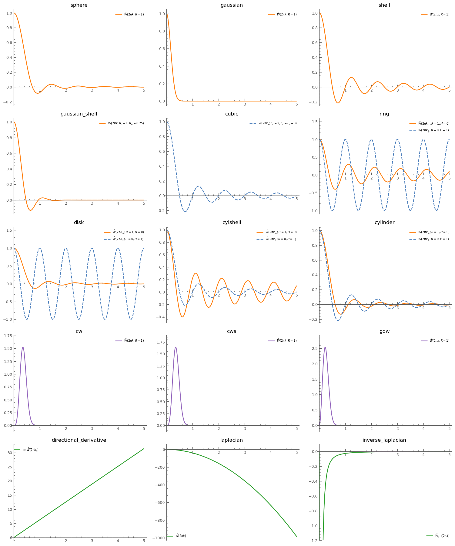
Appendix. Fourier-Space Sketches of Built-In Windows#
This appendix generates one standalone Fourier-space sketch for each built-in PyHermes window. All curves are evaluated from pyhermes.utils.window_functions.WINDOW_TYPE_DICT.
[15]:
from pyhermes.utils.window_functions import WINDOW_TYPE_DICT
import matplotlib.pyplot as plt
from matplotlib.ticker import AutoMinorLocator, MultipleLocator

k = np.linspace(0.0, 5.0, 1600)
zero = np.zeros_like(k)
radial_cut = (k, zero, zero)
parallel_cut = (zero, zero, k)

R_wavelet = 1.0
los_z = (0.0, 0.0, 1.0)
perp_args = (1.0, 0.0, *los_z)
parallel_args = (0.0, 1.0, *los_z)

window_plot_specs = [
    {
        "name": "sphere",
        "curves": [
            {"label": r"$\hat W(2\pi k; R=1)$", "cut": radial_cut, "args": (1.0,), "color": "#ff7f0e", "ls": "-"},
        ],
        "ylim": (-0.25, 1.05),
    },
    {
        "name": "gaussian",
        "curves": [
            {"label": r"$\hat W(2\pi k; R=1)$", "cut": radial_cut, "args": (1.0,), "color": "#ff7f0e", "ls": "-"},
        ],
        "ylim": (-0.05, 1.05),
    },
    {
        "name": "shell",
        "curves": [
            {"label": r"$\hat W(2\pi k; R=1)$", "cut": radial_cut, "args": (1.0,), "color": "#ff7f0e", "ls": "-"},
        ],
        "ylim": (-0.25, 1.05),
    },
    {
        "name": "gaussian_shell",
        "curves": [
            {"label": r"$\hat W(2\pi k; R_s=1,R_g=0.25)$", "cut": radial_cut, "args": (1.0, 0.25), "color": "#ff7f0e", "ls": "-"},
        ],
        "ylim": (-0.18, 1.05),
    },
    {
        "name": "cubic",
        "curves": [
            {"label": r"$\hat W(2\pi k_x; L_x=2,L_y=L_z=0)$", "cut": radial_cut, "args": (2.0, 0.0, 0.0), "color": "#4f81bd", "ls": "--"},
        ],
        "ylim": (-0.25, 1.05),
    },
    {
        "name": "ring",
        "curves": [
            {"label": r"$\hat W(2\pi k_{\perp}; R=1,H=0)$", "cut": radial_cut, "args": perp_args, "color": "#ff7f0e", "ls": "-"},
            {"label": r"$\hat W(2\pi k_{\parallel}; R=0,H=1)$", "cut": parallel_cut, "args": parallel_args, "color": "#4f81bd", "ls": "--"},
        ],
        "ylim": (-1.1, 1.6),
    },
    {
        "name": "disk",
        "curves": [
            {"label": r"$\hat W(2\pi k_{\perp}; R=1,H=0)$", "cut": radial_cut, "args": perp_args, "color": "#ff7f0e", "ls": "-"},
            {"label": r"$\hat W(2\pi k_{\parallel}; R=0,H=1)$", "cut": parallel_cut, "args": parallel_args, "color": "#4f81bd", "ls": "--"},
        ],
        "ylim": (-1.1, 1.6),
    },
    {
        "name": "cylshell",
        "curves": [
            {"label": r"$\hat W(2\pi k_{\perp}; R=1,H=0)$", "cut": radial_cut, "args": perp_args, "color": "#ff7f0e", "ls": "-"},
            {"label": r"$\hat W(2\pi k_{\parallel}; R=0,H=1)$", "cut": parallel_cut, "args": parallel_args, "color": "#4f81bd", "ls": "--"},
        ],
        "ylim": (-0.5, 1.05),
    },
    {
        "name": "cylinder",
        "curves": [
            {"label": r"$\hat W(2\pi k_{\perp}; R=1,H=0)$", "cut": radial_cut, "args": perp_args, "color": "#ff7f0e", "ls": "-"},
            {"label": r"$\hat W(2\pi k_{\parallel}; R=0,H=1)$", "cut": parallel_cut, "args": parallel_args, "color": "#4f81bd", "ls": "--"},
        ],
        "ylim": (-0.25, 1.05),
    },
    {
        "name": "cw",
        "curves": [
            {"label": r"$\hat W(2\pi k; R=1)$", "cut": radial_cut, "args": (R_wavelet,), "color": "#9467bd", "ls": "-"},
        ],
    },
    {
        "name": "cws",
        "curves": [
            {"label": r"$\hat W(2\pi k; R=1)$", "cut": radial_cut, "args": (R_wavelet,), "color": "#9467bd", "ls": "-"},
        ],
    },
    {
        "name": "gdw",
        "curves": [
            {"label": r"$\hat W(2\pi k; R=1)$", "cut": radial_cut, "args": (R_wavelet,), "color": "#9467bd", "ls": "-"},
        ],
    },
    {
        "name": "directional_derivative",
        "curves": [
            {"label": r"$\mathrm{Im}\,\hat W(2\pi k_z)$", "cut": parallel_cut, "args": los_z, "color": "#2ca02c", "ls": "-", "component": "imag"},
        ],
        "ylim": (-1.0, 33.0),
        "legend_loc": "upper left",
    },
    {
        "name": "laplacian",
        "curves": [
            {"label": r"$\hat W(2\pi k)$", "cut": radial_cut, "args": (), "color": "#2ca02c", "ls": "-"},
        ],
        "ylim": (-1030.0, 60.0),
        "legend_loc": "lower left",
    },
    {
        "name": "inverse_laplacian",
        "curves": [
            {"label": r"$\hat W_{\nabla^{-2}}(2\pi k)$", "cut": radial_cut, "args": (), "color": "#2ca02c", "ls": "-"},
        ],
        "ylim": (-1.2, 0.1),
        "legend_loc": "lower right",
    },
]
[16]:
with plt.rc_context({
    "font.family": "DejaVu Sans",
    "mathtext.fontset": "dejavusans",
    "axes.linewidth": 0.8,
    "xtick.color": "0.35",
    "ytick.color": "0.35",
}):
    fig, axes = plt.subplots(5, 3, figsize=(15.0, 18.0), facecolor="white")

    for ax, spec in zip(axes.flat, window_plot_specs):
        fn = WINDOW_TYPE_DICT[spec["name"]]
        finite_values = []

        for curve in spec["curves"]:
            kx_values, ky_values, kz_values = curve["cut"]
            values = np.array([
                fn(float(kx), float(ky), float(kz), *curve["args"])
                for kx, ky, kz in zip(kx_values, ky_values, kz_values)
            ])
            y = np.imag(values) if curve.get("component") == "imag" else np.real(values)
            ax.plot(
                k,
                y,
                color=curve["color"],
                lw=1.8,
                ls=curve["ls"],
                label=curve["label"],
                solid_capstyle="butt",
                dash_capstyle="butt",
            )
            finite_values.extend(y[np.isfinite(y)])

        ax.set_xlim(-0.1, 5.1)
        if "ylim" in spec:
            ax.set_ylim(*spec["ylim"])
        else:
            finite_values = np.asarray(finite_values)
            ymin = float(np.nanmin(finite_values))
            ymax = float(np.nanmax(finite_values))
            yrange = ymax - ymin
            if yrange == 0.0:
                yrange = max(abs(ymin), 1.0)
            ax.set_ylim(ymin - 0.08 * yrange, ymax + 0.15 * yrange)

        ax.spines["left"].set_position(("data", 0.0))
        ax.spines["bottom"].set_position(("data", 0.0))
        ax.spines["right"].set_visible(False)
        ax.spines["top"].set_visible(False)
        ax.spines["left"].set_color("0.35")
        ax.spines["bottom"].set_color("0.35")

        ax.set_xticks(np.arange(1, 6, 1))
        ax.xaxis.set_minor_locator(MultipleLocator(0.2))
        ax.yaxis.set_minor_locator(AutoMinorLocator(5))
        ax.tick_params(axis="both", which="major", direction="in", length=6, width=0.8, labelsize=9)
        ax.tick_params(axis="both", which="minor", direction="in", length=3, width=0.6)
        ax.grid(False)
        ax.set_title(spec["name"], fontsize=12, pad=6)

        ax.legend(
            frameon=False,
            loc=spec.get("legend_loc", "upper right"),
            fontsize=7,
            handlelength=2.2,
            borderaxespad=0.4,
        )

    fig.tight_layout(pad=0.6, h_pad=1.0, w_pad=1.2)
    plt.show()
Next steps#
Projection and windows are the common foundation for the remaining examples. Continue with physical_fields.ipynb to apply differential and inverse-Laplacian operators, counting.ipynb to sample one-point distributions, or corr2pcf.ipynb followed by corr3pcf.ipynb for correlation statistics.